| L5_CD | L3_CD | L3_EN | L1_CD | L1_EN |
|---|---|---|---|---|
| 01290 | 012 | Growing of perennial crops | A | Agriculture, forestry and fishing |
| 15110 | 151 | Tanning and dressing of leather; manufacture of luggage, handbags,saddlery and harness; dressing and dyeing of fur | C | Manufacturing |
| 27900 | 279 | Manufacture of other electrical equipment | C | Manufacturing |
| 38211 | 382 | Waste treatment and disposal | E | Water supply; sewerage; waste management and remediation activities |
| 46710 | 467 | Other specialised wholesale | G | Wholesale and retail trade; repair of motor vehicles and motorcycles |
| 47230 | 472 | Retail sale of food, beverages and tobacco in specialised stores | G | Wholesale and retail trade; repair of motor vehicles and motorcycles |
| 47252 | 472 | Retail sale of food, beverages and tobacco in specialised stores | G | Wholesale and retail trade; repair of motor vehicles and motorcycles |
| 45202 | 452 | Maintenance and repair of motor vehicles | G | Wholesale and retail trade; repair of motor vehicles and motorcycles |
| 46120 | 461 | Wholesale on a fee or contract basis | G | Wholesale and retail trade; repair of motor vehicles and motorcycles |
| 77296 | 772 | Renting and leasing of personal and household goods | N | Administrative and support service activities |
3 Data Analytics Report
Keywords
Occupational Accidents, Workplace Accidents, Accidents at work, Workplace injuries, Determinants, Factors, Cost, Occupational Safety, Occupational Risk, Commuting Accidents, Accident Frequency, Accident Severity
3.1 Representativeness of the employer data
Unlike National Social Security Office (NSSO) and Federaal agentschap voor beroepsrisico’s (FEDRIS), two Belgian federal services, Liantis does not have access to employment and Occupational Accident (OA) data of the full Belgian population. Therefore, we need to assess the representativeness of the Liantis employer data in comparison to the full Belgian employer population.
Since Liantis has access to basic Crossroads Bank for Enterprises (KBO in Dutch) (CBE) information for all Belgian employers (e.g. Belgian version of the the Europese activiteitennomenclatuur (NACE) (NACE-BEL) 2008 classification and municipality per CBE number) it is possible to make the comparison with the Liantis External Service for Prevention and Protection at work (EDPB in Dutch) (ESPP) and Payroll Services (PS) mutual employers, for which the same information is present together with employment and OA data. This will allow us to make a representative sample of the Liantis mutual customers and to correct for representativeness in the further analysis when needed.
As the Liantis PS and ESPP mutual customers are primarely located in Flanders, we will focus on the representativeness of the Liantis mutual customers in Flanders.
We start with loading a summary table of the NACE-BEL 2008 structure. The table (in long format) contains all codes (in 5 levels) with their corresponding labels in four languages (Dutch, French, English and German).
- level 1: sections, of which there are 21, identified by alphabetical letters (A to U)
- level 2: divisions, of which there are 88, identified by two-digit numerical codes ranging from 01 to 99
- level 3: groups, of which there are 272, identified by three-digit numerical codes ranging from from 011 to 990
- level 4: classes, of which there are 615, identified by four-digit numerical codes ranging from 0111 to 9900
- level 5: subclasses, of which there are 943, identified by five-digit numerical codes ranging from 01110 to 99000
We restructure this table into a hierarchical (broad) format. This will allow us to easily join more general codes (level 3 and level 1) to more specific codes (level 5) present in our data.
Table 3.1 shows a sample of ten rows of the codes and labels at level 5,3 and 1.
In a next step, we load a summary table ‘datam’ in which all Belgian municipalities with corresponding postal code (see Section 2.7.3.3) are mapped to their Province and Region.
Once we have the sector (NACE-BEL 2008 codes) and geographical (postal codes, Nationaal Instituut voor de Statistiek (NIS) codes & municipalities) classification systems available, we load a table in which all Belgian active employers with NSSO activities (paid employees) are present with their CBE number, NACE-BEL 2008 level 5 code and postal code. This information is obtained trough the Liantis CBE-COPY-SERVICE which synchronizes a few basic elements from the CBE register to the Liantis data lake. Data from NACE-BEL 2008 classification system ‘nacesum’ as wel as the geographical information ‘datam’ are left joined. The object was generated and stored 09/04/2025 with the name ‘crbsnapshot’. See ‘functions/constructionCBE_datasource.R’ for details.
We load the object, filter on Flanders, and group by province and level 3 NACE-BEL 2008 code to count the number of employers per province and level 3 NACE-BEL 2008 code.
Table 3.2 shows the top ten rows of this counts as an example.
| Region | Province | L3_CD | ncbe |
|---|---|---|---|
| Vlaanderen | Antwerpen | 011 | 293 |
| Vlaanderen | Antwerpen | 012 | 97 |
| Vlaanderen | Antwerpen | 013 | 67 |
| Vlaanderen | Antwerpen | 014 | 267 |
| Vlaanderen | Antwerpen | 015 | 42 |
| Vlaanderen | Antwerpen | 016 | 82 |
| Vlaanderen | Antwerpen | 021 | 6 |
| Vlaanderen | Antwerpen | 022 | 5 |
| Vlaanderen | Antwerpen | 024 | 1 |
| Vlaanderen | Antwerpen | 031 | 1 |
We take the Liantis ESPP and PS mutual customers and classify them into two segments: smaller companies up to 49 employees and larger companies from 50 employees on. The result is shown in Table 3.3.
| segment | n | percentage |
|---|---|---|
| small | 47394 | 99.1 |
| large | 426 | 0.9 |
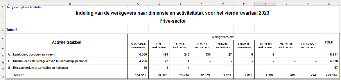
In the Liantis dataset of mutual customers, only 0.9% of mutual employers are considered large employers. This is lower than the 3.4% calculated from the number of employers, defined under “De werkgever” in the last quarter of 2023, as data from ‘Employment_valAANTALW_NL_20234.xlsx’ (downloaded from the archive, sheet 2 private sector, show (<50 (221545) and \(\geq\) 50 (7831), Figure 3.1). Hence, it will also be a good idea to include also this criterion in the representativeness check.
Within the mutual customers, we clean the NACE-BEL 2008 codes where necessary (removal of dots, adding of leading zero’s), join the structured NACE-BEL 2008 information and the geographical information. Subsequently we filter on Flanders (Liantis PS has a much smaller portion of customers in Wallonia and Brussels than Liantis ESPP).
If we look at the number of Liantis mutual ESPP and PS customers per Flemish province and NACE-BEL 2008 level 1 sector in Table 3.4, we see that there are a few sectors with very few customers (B, D, E, O, T & U). If we want to report on employers distributed representatively across Flemish provinces and NACE-BEL 2008 level 1 sectors, those sectors will need to be filtered out because of lack of representativeness.
| Antwerpen | Limburg | Oost-Vlaanderen | Vlaams-Brabant | West-Vlaanderen | |
|---|---|---|---|---|---|
| A | 86 | 76 | 85 | 60 | 458 |
| B | 0 | 2 | 0 | 0 | 0 |
| C | 372 | 404 | 390 | 247 | 1396 |
| D | 3 | 2 | 0 | 2 | 3 |
| E | 12 | 16 | 12 | 7 | 57 |
| F | 1287 | 1187 | 1007 | 879 | 3134 |
| G | 1603 | 1442 | 1219 | 1083 | 3747 |
| H | 263 | 172 | 239 | 192 | 552 |
| I | 1340 | 963 | 1034 | 940 | 3151 |
| J | 166 | 100 | 157 | 141 | 219 |
| K | 212 | 132 | 193 | 158 | 491 |
| L | 143 | 131 | 104 | 112 | 448 |
| M | 539 | 436 | 461 | 365 | 1117 |
| N | 357 | 265 | 321 | 302 | 885 |
| O | 0 | 5 | 8 | 1 | 8 |
| P | 65 | 55 | 80 | 33 | 198 |
| Q | 312 | 294 | 265 | 232 | 776 |
| R | 169 | 122 | 136 | 108 | 284 |
| S | 471 | 372 | 381 | 307 | 986 |
| T | 29 | 15 | 13 | 23 | 56 |
| U | 2 | 0 | 0 | 0 | 0 |
Data Quality Alert: some (primarly public) sectors have to be filtered out from further analysis because of lack of representativeness
The combined Belgian workforce and employer presence in sectors B, D, E, O, U, and T is predominantly associated with the public sector. This is primarily due to the substantial representation of sectors O (public administration) and U (international organisations), despite the partially private nature of sectors B, D, and E. Given that Liantis primarily serves private sector employers, it is unsurprising that these sectors are underrepresented in the Liantis database. This underrepresentation may introduce bias if these sectors are included in the analysis. Therefore, to safeguard the accuracy and reliability of our findings, we have chosen to exclude these sectors from further analysis.
After filtering out the sectors B, D, E, O, T, U (respectively Mining and quarrying; Electricity, gas, steam and air conditioning supply; Water supply; sewerage; waste management and remediation activities; Public administration and defence; compulsory social security; Activities of households as employers; undifferentiated goods- and services-producing activities of households for own use; Activities of extraterritorial organisations and bodies), no missing NACE-BEL 2008 level 1 or postal codes remain.
An overview of NACE-BEL 2008 level 1 sectors labels and there meaning (in English and Dutch) can be found in Table 3.5.
| NID1 | SECTIONS | SECTIES |
|---|---|---|
| A | Agriculture, forestry and fishing | Landbouw, bosbouw en visserij |
| B | Mining and quarrying | Winning van delfstoffen |
| C | Manufacturing | Industrie |
| D | Electricity, gas, steam and air conditioning supply | Productie en distributie van elektriciteit, gas, stoom en gekoelde lucht |
| E | Water supply; sewerage; waste management and remediation activities | Distributie van water; afval- en afvalwaterbeheer en sanering |
| F | Construction | Bouwnijverheid |
| G | Wholesale and retail trade; repair of motor vehicles and motorcycles | Groot- en detailhandel; reparatie van auto’s en motorfietsen |
| H | Transportation and storage | Vervoer en opslag |
| I | Accommodation and food service activities | Verschaffen van accommodatie en maaltijden |
| J | Information and communication | Informatie en communicatie |
| K | Financial and insurance activities | Financiële activiteiten en verzekeringen |
| L | Real estate activities | Exploitatie van en handel in onroerend goed |
| M | Professional, scientific and technical activities | Vrije beroepen en wetenschappelijke en technische activiteiten |
| N | Administrative and support service activities | Administratieve en ondersteunende diensten |
| O | Public administration and defence; compulsory social security | Openbaar bestuur en defensie; verplichte sociale verzekeringen |
| P | Education | Onderwijs |
| Q | Human health and social work activities | Menselijke gezondheidszorg en maatschappelijke dienstverlening |
| R | Arts, entertainment and recreation | Kunst, amusement en recreatie |
| S | Other service activities | Overige diensten |
| T | Activities of households as employers; undifferentiated goods- and services-producing activities of households for own use | Huishoudens als werkgever; niet-gedifferentieerde productie van goederen en diensten door huishoudens voor eigen gebruik |
| U | Activities of extraterritorial organisations and bodies | Extraterritoriale organisaties en lichamen |
Since we had customer data and CBE data available at NACE-BEL 2008 level 3 and postal code, but we want to take a representative sample at NACE-BEL 2008 level 1 and Flemish province, we further summarise our employer data to level 1 and Province.
The first ten rows of the result of this summarization are shown in Table 3.6.
| Region | Province | NID1 | L1_EN | nLiantis | nCBE |
|---|---|---|---|---|---|
| Vlaanderen | Antwerpen | A | Agriculture, forestry and fishing | 86 | 859 |
| Vlaanderen | Antwerpen | C | Manufacturing | 370 | 2200 |
| Vlaanderen | Antwerpen | F | Construction | 1287 | 4783 |
| Vlaanderen | Antwerpen | G | Wholesale and retail trade; repair of motor vehicles and motorcycles | 1603 | 8797 |
| Vlaanderen | Antwerpen | H | Transportation and storage | 263 | 1951 |
| Vlaanderen | Antwerpen | I | Accommodation and food service activities | 1340 | 4676 |
| Vlaanderen | Antwerpen | J | Information and communication | 165 | 1536 |
| Vlaanderen | Antwerpen | K | Financial and insurance activities | 212 | 1243 |
| Vlaanderen | Antwerpen | L | Real estate activities | 143 | 1053 |
| Vlaanderen | Antwerpen | M | Professional, scientific and technical activities | 539 | 3828 |
Subsequently, we calculate the necessary proportions to be able compile a list from which we can randomly draw a sample.
- propLiantis is the percentage of companies within Liantis in the combination of Flemish province and NACE-BEL 2008 1 level
- propCBE is the percentage of companies within the CBE in the combination of Flemish province and NACE-BEL 2008 1 level
- ratioSampleCBE is the ratio of the proportions within the sample and the CBE and should be around 1 to be representative. Ratios much larger than 1 indicate an over-representation in our customer base, ratios much smaller than 1 indicate an under-representation in our customer base
- if we propose to construct a representative sample of 10000 employers, we can calculate the number of companies to be sampled per province and NACE-BEL 2008 level 1 sector combination (and size <50 or \(\geq\) 50 employees).
This gives us the necessary proportions and numbers to sample over the combinations of Flemish provinces and NACE-BEL 2008 1 levels. The first and last five rows as shown as an example in Table 3.7.
| Province | NID1 | nLiantis | nCBE | nSample | propLiantis | propCBE | propSample | ratioLiantisCBE | ratioSampleCBE | sampleOK |
|---|---|---|---|---|---|---|---|---|---|---|
| West-Vlaanderen | I | 3151 | 3612 | 274 | 0.074 | 0.027 | 0.027 | 2.7 | 1 | TRUE |
| West-Vlaanderen | S | 986 | 1115 | 84 | 0.023 | 0.008 | 0.008 | 2.7 | 1 | TRUE |
| West-Vlaanderen | P | 198 | 245 | 19 | 0.005 | 0.002 | 0.002 | 2.5 | 1 | TRUE |
| West-Vlaanderen | F | 3134 | 4134 | 313 | 0.074 | 0.031 | 0.031 | 2.3 | 1 | TRUE |
| West-Vlaanderen | G | 3747 | 5829 | 442 | 0.088 | 0.044 | 0.044 | 2.0 | 1 | TRUE |
| Vlaams-Brabant | A | 60 | 473 | 36 | 0.001 | 0.004 | 0.004 | 0.4 | 1 | TRUE |
| Vlaams-Brabant | P | 33 | 258 | 20 | 0.001 | 0.002 | 0.002 | 0.4 | 1 | TRUE |
| Antwerpen | A | 86 | 859 | 65 | 0.002 | 0.007 | 0.007 | 0.3 | 1 | TRUE |
| Antwerpen | J | 165 | 1536 | 116 | 0.004 | 0.012 | 0.012 | 0.3 | 1 | TRUE |
| Limburg | A | 75 | 759 | 57 | 0.002 | 0.006 | 0.006 | 0.3 | 1 | TRUE |
Next, we generate the file ‘datas’ with the representative sample of employers and save it.
In the table Table 3.8 we show the result of the sampling procedure on the mutual customers.
| variable | Province | A | C | F | G | H | I | J | K | L | M | N | P | Q | R | S |
|---|---|---|---|---|---|---|---|---|---|---|---|---|---|---|---|---|
| nKBO | Antwerpen | 862.00 | 2376.00 | 4783.00 | 8797.00 | 1968.00 | 4676.00 | 1550.00 | 1253.00 | 1053.00 | 3828.00 | 1986.00 | 431.00 | 2070.00 | 1090.00 | 1554.00 |
| nSAM | Antwerpen | 63.00 | 164.00 | 360.00 | 656.00 | 147.00 | 348.00 | 113.00 | 91.00 | 80.00 | 284.00 | 149.00 | 35.00 | 156.00 | 83.00 | 112.00 |
| percKBO | Antwerpen | 0.65 | 1.78 | 3.59 | 6.61 | 1.48 | 3.51 | 1.16 | 0.94 | 0.79 | 2.87 | 1.49 | 0.32 | 1.55 | 0.82 | 1.17 |
| percSAM | Antwerpen | 0.63 | 1.64 | 3.60 | 6.56 | 1.47 | 3.48 | 1.13 | 0.91 | 0.80 | 2.84 | 1.49 | 0.35 | 1.56 | 0.83 | 1.12 |
| nKBO | Limburg | 759.00 | 1402.00 | 2849.00 | 3788.00 | 598.00 | 2053.00 | 414.00 | 583.00 | 305.00 | 1449.00 | 802.00 | 200.00 | 1008.00 | 386.00 | 753.00 |
| nSAM | Limburg | 57.00 | 100.00 | 208.00 | 282.00 | 46.00 | 151.00 | 31.00 | 44.00 | 23.00 | 109.00 | 62.00 | 19.00 | 74.00 | 29.00 | 54.00 |
| percKBO | Limburg | 0.57 | 1.05 | 2.14 | 2.84 | 0.45 | 1.54 | 0.31 | 0.44 | 0.23 | 1.09 | 0.60 | 0.15 | 0.76 | 0.29 | 0.57 |
| percSAM | Limburg | 0.57 | 1.00 | 2.08 | 2.82 | 0.46 | 1.51 | 0.31 | 0.44 | 0.23 | 1.09 | 0.62 | 0.19 | 0.74 | 0.29 | 0.54 |
| nKBO | Oost-Vlaanderen | 709.00 | 2207.00 | 4796.00 | 6092.00 | 1275.00 | 3121.00 | 926.00 | 1032.00 | 645.00 | 2773.00 | 1473.00 | 349.00 | 1659.00 | 838.00 | 1256.00 |
| nSAM | Oost-Vlaanderen | 50.00 | 159.00 | 352.00 | 458.00 | 98.00 | 233.00 | 69.00 | 75.00 | 47.00 | 207.00 | 104.00 | 30.00 | 123.00 | 61.00 | 92.00 |
| percKBO | Oost-Vlaanderen | 0.53 | 1.66 | 3.60 | 4.57 | 0.96 | 2.34 | 0.70 | 0.77 | 0.48 | 2.08 | 1.11 | 0.26 | 1.25 | 0.63 | 0.94 |
| percSAM | Oost-Vlaanderen | 0.50 | 1.59 | 3.52 | 4.58 | 0.98 | 2.33 | 0.69 | 0.75 | 0.47 | 2.07 | 1.04 | 0.30 | 1.23 | 0.61 | 0.92 |
| nKBO | Vlaams-Brabant | 473.00 | 918.00 | 2982.00 | 4628.00 | 1284.00 | 2490.00 | 882.00 | 565.00 | 475.00 | 2096.00 | 1224.00 | 272.00 | 1141.00 | 524.00 | 1040.00 |
| nSAM | Vlaams-Brabant | 35.00 | 60.00 | 221.00 | 344.00 | 96.00 | 182.00 | 61.00 | 42.00 | 35.00 | 152.00 | 87.00 | 20.00 | 91.00 | 40.00 | 77.00 |
| percKBO | Vlaams-Brabant | 0.36 | 0.69 | 2.24 | 3.47 | 0.96 | 1.87 | 0.66 | 0.42 | 0.36 | 1.57 | 0.92 | 0.20 | 0.86 | 0.39 | 0.78 |
| percSAM | Vlaams-Brabant | 0.35 | 0.60 | 2.21 | 3.44 | 0.96 | 1.82 | 0.61 | 0.42 | 0.35 | 1.52 | 0.87 | 0.20 | 0.91 | 0.40 | 0.77 |
| nKBO | West-Vlaanderen | 1170.00 | 2538.00 | 4134.00 | 5829.00 | 1079.00 | 3612.00 | 472.00 | 1003.00 | 796.00 | 2129.00 | 1352.00 | 245.00 | 1336.00 | 596.00 | 1124.00 |
| nSAM | West-Vlaanderen | 85.00 | 206.00 | 319.00 | 442.00 | 81.00 | 272.00 | 33.00 | 72.00 | 57.00 | 162.00 | 110.00 | 43.00 | 158.00 | 46.00 | 83.00 |
| percKBO | West-Vlaanderen | 0.88 | 1.91 | 3.10 | 4.38 | 0.81 | 2.71 | 0.35 | 0.75 | 0.60 | 1.60 | 1.02 | 0.18 | 1.00 | 0.45 | 0.84 |
| percSAM | West-Vlaanderen | 0.85 | 2.06 | 3.19 | 4.42 | 0.81 | 2.72 | 0.33 | 0.72 | 0.57 | 1.62 | 1.10 | 0.43 | 1.58 | 0.46 | 0.83 |
The result of the procedure was tested with a Chi-squared test of independence. Effect sizes were labelled following Funder’s (2019) recommendations. The Pearson’s Chi-squared test of independence between sample and CBE suggests that the effect is statistically not significant (\(\chi^2 = 55.59\), \(p = 0.946\)).
From the representative sample of 10000 employers we can extract the CBE number, and subsequently label which employers in the complete dataset of mutual ESPP and PS customers make part of this representative subset (for NACE-BEL 2008 level 1 code, Flemish province and size <50 or \(\geq\) 50 employees) and which do not.
At this point, it is possible to indicate which OAs took place in the representative subset and which took place in other companies as well as to examine which variables which might be influenced. An example is shown in Table 3.9: the seriousness of an OA does not seem to differ between the complement and the representative subset, but biological sex does. Our raw dataset contains a lot more male workers experiencing an OA, but in a representative subset biological sex is more equally balanced. Hence, correcting for representativeness is important when analysing OAs.
| category | OAnotinrep | OAinrep | percOAnotinrep | perOAinrep |
|---|---|---|---|---|
| total | 188998 | 27948 | 87.12 | 12.88 |
| normal oa | 121189 | 23931 | 95.41 | 95.54 |
| potential serious oa | 1082 | 219 | 0.85 | 0.87 |
| serious oa | 4753 | 899 | 3.74 | 3.59 |
| F | 44668 | 11857 | 35.24 | 47.39 |
| M | 82070 | 13165 | 64.76 | 52.61 |
A representative sample of 10,000 employers
We were able to draw a representative sample of 10,000 employers based on the following characteristics:
- Province: representative across the Flemish Region (excluding Brussels),
- Sector: classified according to the NACE level 1 code (excluding sectors B, D, E, O, U, and T),
- Company size: categorized as either fewer than 50 employees or 50 employees and more,
- Establishment count: the number of companies established within each unique combination of these factors (province × sector × size) was taken into account to ensure proportional representation.
To account for potential differences in outcomes due to representativeness issues, a binary variable indicating whether an observation belongs to the representative sample can be included in the models.
3.2 Statistical methodology
The data analysis is conducted in two stages. First, descriptive statistics of the determinants are presented. When applicable, external references (e.g., NSSO, FEDRIS) are included. In the second stage, each determinant is modelled in relation to various outcome variables (see Section 1.2). Modelling is done in a univariable (per single determinant, see Section 3.4) as well as a multivariable (all determinants combined, see Section 3.5) context.
3.2.1 Descriptives
Stage one presents descriptive data on determinants related to OAs. External sources, such as NSSO and FEDRIS, provide standardized classifications for determinants attributable to both employees and employers (age, gender, nsso category, sector,…). This data, being publicly accessible through statistical quarter or year reports, is collected and structured into categories to support comparative analysis.
Where applicable, data is presented for all employees, combining public and private sectors, as well as for private sector employees separately. The numbers include total OAs, with a further breakdown into commuting and workplace accidents. When possible, three tables are provided for each category (total, commuting, and workplace accidents), each shown both in absolute numbers and as percentages across categories. For comparability, a representative sample of mutual Liantis ESPP and PS customers was created. Based on census data, companies were sampled by sector (NACE-BEL 2008 section), Flemish province, and employee count (<50 or \(\geq\) 50). All relevant employee records from these firms, over the relevant time period, are included.
The descriptive tables include a maximum of eight columns, each representing a specific set.
- category: the various categories of the determinant.
- Rijksdienst voor Sociale Zekerheid (RSZ) all: aggregated totals or percentages of employees in both public and private sectors, based on quarterly data from 2014 to 2023 from the NSSO (in Dutch RSZ). This acts as an external reference.
- RSZ private: aggregated totals or percentages of employees in the private sector, based on quarterly data from 2014 to 2023 from the NSSO (in Dutch RSZ. This acts as an external reference.
- Liantis all: aggregated totals or percentages of employees from Liantis client employers, specifically those using both PS and ESPP services in the private sector, based on monthly data from 2014 to 2023.
- FEDRIS All: notifications of OAs in the private sector, as reported to FEDRIS, combining commuting and workplace accidents, aggregated over the years 2014 to 2023. This acts as an external reference.
- TotalNot: OA notifications among all Liantis customers using ESPP services in the private sector, aggregated over the years 2014 to 2023.
- TotalNotMut: OA notifications among mutual Liantis customers using both PS and ESPP services in the private sector, aggregated over the years 2014 to 2023.
- TotalNotMutRep: OA notifications among mutual Liantis customers using both PS and ESPP services in the private sector, limited to a representative sample of employers (by Flemish province, sector, and company size), aggregated over the years 2014 to 2023.
3.2.2 Modelling
3.2.2.1 Datasets
The datasets used for modelling include variables such as company identifiers and individual identifiers, year, month, and the respective outcome variable. All statistical models were constructed using the glmmTMB package (Brooks et al., 2017) using approximations to estimate the Intraclass Correlation Coefficient (ICC) where necessary, based on methods proposed by Nakagawa et al. (2017). Only mutual Liantis ESPP and PS customers are included over the respective timeframe. Observations corresponding to individuals employed by these companies during the relevant time periods are included. A representative sample, aligned with the one used in the descriptive statistics, is present as a subset. An additional variable identifies whether an observation is part of this sample or not, to account for potential differences in outcomes.
It is important to note that the inclusion of this variable to correct for representativeness (as a fixed effect) did not significantly alter the effect sizes or significance levels of the other determinants, suggesting that its presence does not bias the results found.
Fallacies
When interpreting our findings, it is essential to be mindful of the ecological and atomistic fallacies, which can lead to incorrect conclusions if inferences are made at the wrong level of analysis. The ecological fallacy involves applying group-level associations to individuals, while the atomistic fallacy occurs when individual-level relationships are assumed to hold at the group level. These fallacies are particularly relevant in our study, where both individual and organisational-level data are analysed.
For example, at the individual level, we find that younger workers are more likely to experience occupational accidents. However, at the group level, organisations with a higher proportion of younger employees tend to have lower rates of occupational accidents. This apparent contradiction illustrates how relationships can differ, or even reverse, depending on the level of analysis. One possible explanation is that organisations employing more young workers may also have better safety cultures, more dynamic work environments, or more proactive prevention policies, which mitigate risk at the group level despite individual vulnerabilities. This example underscores the importance of aligning interpretations with the appropriate level of data and avoiding simplistic generalizations across levels. Recognizing these fallacies helps ensure that conclusions are both accurate and contextually valid.
3.2.2.2 Occurence
The first set of models examines the occurrence of OAs. Four models (Model 1, Model 1.1, Model 2 and Model 3) address individual-level outcomes; a fifth one (Model 4) focuses on a company-level outcome. A multilevel modelling approach is generally applied, recognizing the hierarchical structure of the data, where observations are nested within individuals and individuals within companies. Theoretically, this structure would justify a three-level model. However, due to convergence issues encountered during estimation, a two-level model is used instead, with both individual and company-level clustering treated at the same level. For the fifth model (Model 4), a multilevel modelling approach for a company-level ouctome is employed to account for repeated yearly observations at company-level.
- Model 1 (hadOA): likelihood to notify an OA, both commuting and workplace notifications. Each observation represents a specific month for an individual and indicates whether an OA notification was reported during that period in relation to the determinant.
- Model 1.1 (statusOA): likelihood an OA insurer refuses an OA, both commuting and workplace notifications. Each observation represents whether a specific OA notification was refused in relation to the determinant. This dataset is a subset of the dataset used in Model 1 (only workers with OA notifications).
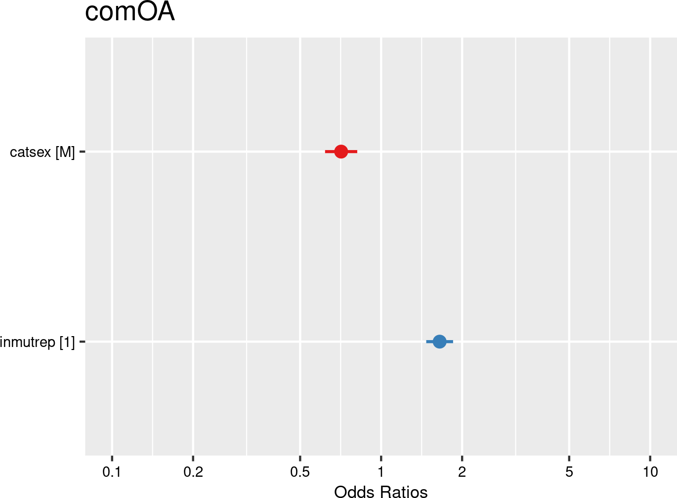
- Model 2 (comOA): likelihood to experience an accepted commuting OA. Each observation represents a specific month for an individual and indicates whether an accepted OA notification during commuting was noted during that period in relation to the determinant. This dataset is similar to the dataset used in Model 1, but workplace OAs are in this set not counted (since these are non-commuting accidents).
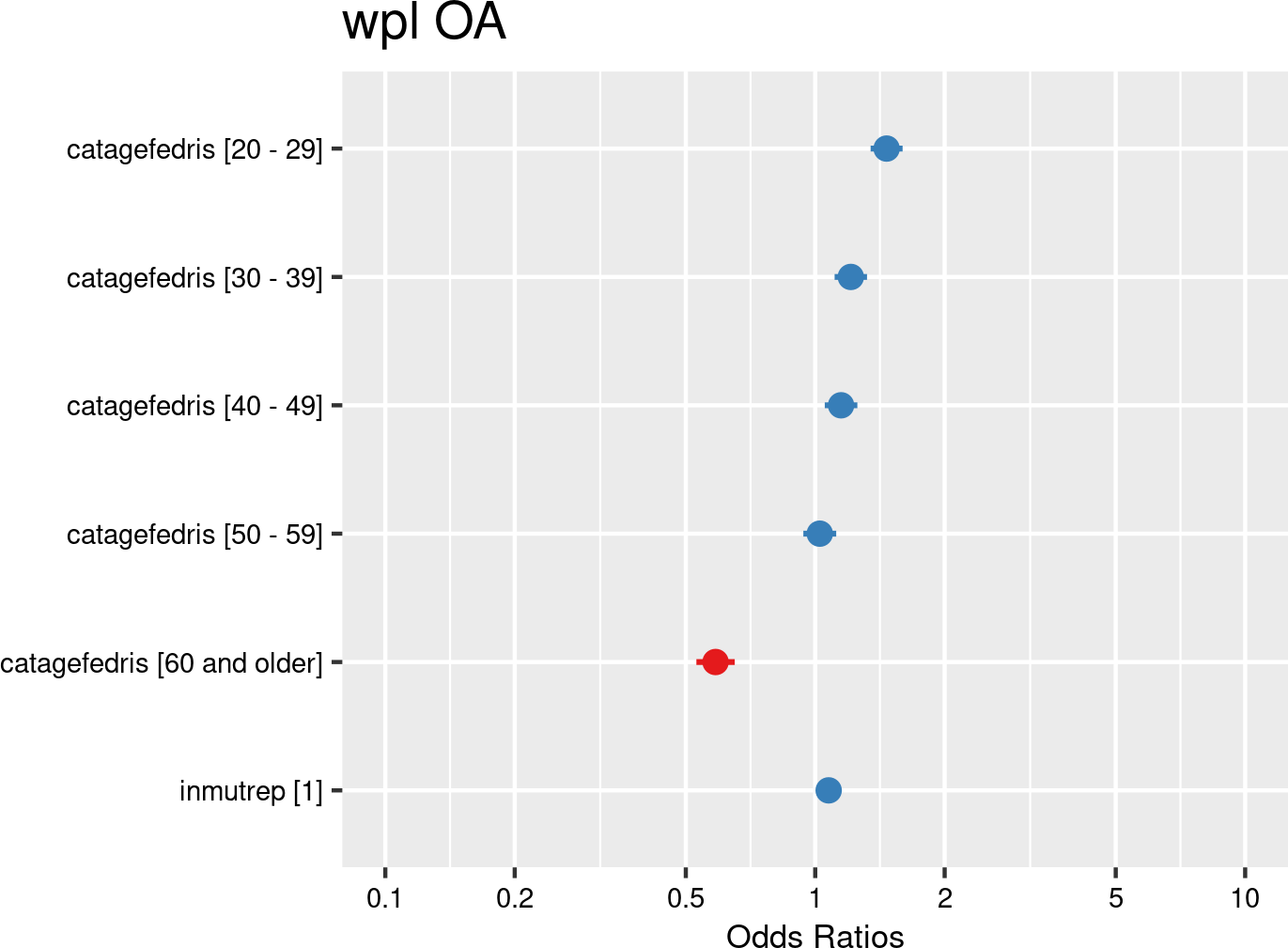
- Model 3 (wplOA): likelihood to experience an accepted workplace OA. Each observation represents a specific month for an individual and indicates whether an accepted OA notification for the workplace was noted during that period in relation to the determinant. This dataset is similar to the dataset used in Model 1, but commuting OAs are in this set not counted (since these are non-workplace accidents).
- Model 4 (freqOA): this model focuses on a company-level outcome: the frequency degree of OAs. This metric is calculated by dividing the number of accepted workplace OAs by the total hours of exposure, multiplied by a constant (1,000,000). Determinants are expressed as fractions (ranging from 0 to 1) representing the proportion of employees in specific categories. For instance, when age is used as a determinant, the workforce is divided into six age groups, and the model includes the proportion of employees (some categories can be left out due to rank deficiency issues). Each observation corresponds to a company, with repeated yearly measures clustered at the company level.
Five models related to occurrence
A series of five models will address the likelihood and frequency of occupational accidents, at both individual and company levels. A multilevel modelling approach is used to account for the hierarchical structure of the data.
3.2.2.3 Severity
The second group of models examines the severity of OAs using individual-level data. The first four models focus on (monthly) individual outcomes, the last two on a (yearly) company level outcome.
The first model (Model 5) models OA seriousness in a two-level structure, treating individual and company clustering equivalently.
The next two (Model 6 and Model 6.1) model absence days. To address the count nature of this number of days as well as overdispersion, a negative binomial distribution is used. Specifically, the NB2 parametrization is applied, where the conditional variance increases quadratically with the mean. This approach offers greater flexibility in modelling scenarios where overdispersion grows with the expected value, making it more appropriate than a Poisson model in this context.
For the fourth model (Model 7), a multilevel modelling approach is applied to account for clustering at the company level, reflecting repeated observations within the same organisational context.
The last two (Model 8 and Model 8.1) shift to company-level outcomes and use multilevel modelling to incorporate repeated yearly observations of company variables. Determinants in this models are operationalized as fractions (ranging from 0 to 1) of employees falling into specific categories. For example, when using age as a determinant, the workforce is divided into six age groups, and the model includes the proportion of employees in each group per company. Observations are thus companies with their fractions. In this model the observations are clustered on a company level to account for repeated measures through time (in maximum the 10 different years of the study between 2014 and 2023).
- Model 5 (seriousOA): chance on a severe accepted workplace OA (see Section 2.10). The binary outcome indicates whether a workplace accident was classified as severe in relation to the determinant. Only workplace OA are considered, as commuting accidents are (according to Belgian law) never to be regarded as serious Liantis database information (in certain cases modified data in comparison with the original relevant notification fields) is used in combination with the original commuting information from the notification the decide on seriousness. Each observation represents a single OA.
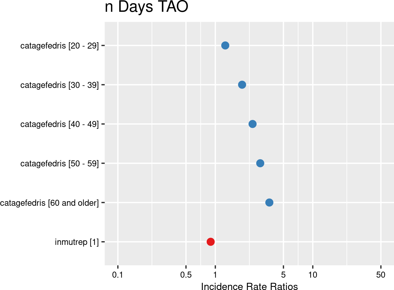
- Model 6 (nDaysTAO): duration of absence. This outcome captures the (validated) number of days an individual is absent due to an OA. Absence duration is operationalized in two ways. This first way reflects validated days of absence, as reported by FEDRIS (and, by extension, insurers), representing officially recognized durations of absence.
- Model 6.1 (lengtecor): duration of absence. This outcome captures the (calculated) number of days an individual is absent due to an OA. Absence duration is operationalized in two ways. This second way reflects duration of absence by using Liantis PS data calculating absence days based on wage codes linked to OAs, offering an alternative measure of absence duration.
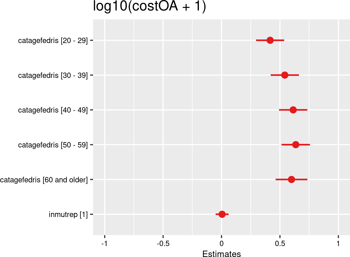
- Model 7 (costOA): cost of OAs. This cost is calculated based on the actual wage expenses incurred during the period of absence, as recorded in payroll data. Each observation represents a single OA, with the corresponding wage cost for the absence period. Since the costs are higly skewed to the right, a log10-transformation is applied to the original cost + €1 (to avoid minus infinity results) to normalize the distribution.
- Model 8 (sevOAval): severity degree (validated days). This collective measure reflects the proportion of the sum of the number of lost calendar days from employees within a company who experienced a workplace OA. The sum of the total number lost calendar days is calculated in two ways. This first way uses the sum of the validated days of absence as reported by FEDRIS (and, by extension, insurers), representing officially recognized durations of absence.
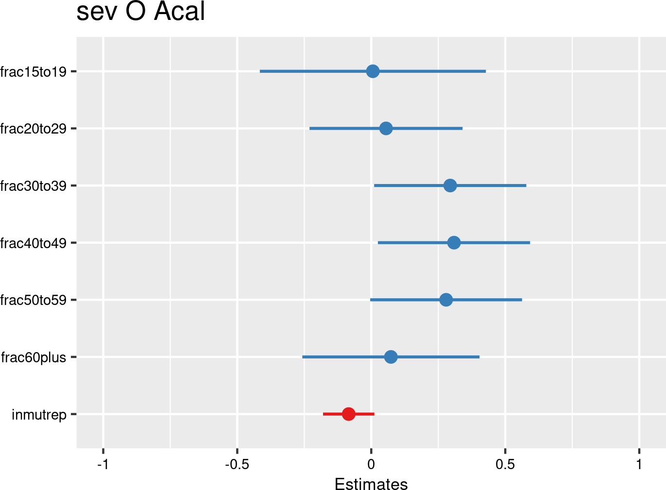
- Model 8.1 (sevOAcal): severity degree (calculated days). This collective measure reflects the proportion of the sum of the number of lost calendar days from employees within a company who experienced an workplace OA. The sum of the total number lost calendar days is calculated in two ways. This second way to operationalize the severity degree is by using payroll-reported days of absence based on wage codes provided through Liantis PS data, offering an alternative measure of absence duration.
Six models related to severity
Six models will address severity of occupational accidents at both individual and company levels. They examine the likelihood of severe accidents, duration of absence, and associated costs, using validated and calculated days absent. A multilevel modelling approach is used to account for the hierarchical structure of the data.
3.3 Outcomes
The outcomes analyzed in this study encompass a range of indicators related to OA and incidents, including:
- notifications;
- accepted accidents;
- commuting accidents;
- workplace accidents;
- frecuency degree;
- seriousness of OA;
- length of absence following an OA;
- cost of OA;
- severity degree.
These outcomes are discussed in detail in Section 3.5, where they are integrated into multivariable models. A key consideration is that many of these outcomes are inherently tied to a temporal dimension (e.g. amount of notifications in a certain month of a given year). As such, providing standalone descriptive statistics outside the modelling context would be both methodologically limiting and potentially misleading.
Additionally, several outcomes, particularly frequency degree and severity degree, are derived measures that rely on assumptions about exposure. These assumptions can vary significantly depending on the chosen methodology. For instance, exposure hours may be estimated using a flat calculation (e.g., standard definition) or derived from actual payroll data, which reflects real-time presence and activity. These methodological choices directly influence the distribution and interpretation of the outcomes, and thus must be considered within the modelling framework.
Another important factor is data completeness. Different models exclude varying subsets of data due to missing values in key variables. This means that the distribution of the final modelled outcomes may differ from the raw distributions, further complicating the presentation of general descriptives.
Taken together, these considerations, temporal dependencies, methodological variability in derived measures, and data exclusions, have led to the decision not to present standalone descriptive statistics for these outcomes in this section. Instead, the outcomes are more appropriately interpreted within the context of the multivariable models, where these complexities are accounted for.
For readers who still like to find some more detailed descriptive statistics on some of the outcomes, we refer to Section 3.4.5.1. In the descriptives section of this univariable analysis by year, counts and percentages are presented for each of the ten years of the study.
Counting and reporting a number of OA per year might not be as simple as it seems
An apparently simple parameter like the number of OA per year can be counted in very different ways:
- a total number of notifications as a proxy for all OAs (last declarations, before any acceptance or refusal, as well commuting as workplace accidents)
- not all those declarations of OAs will be accepted by the insurers
- accepted OAs are further classified for reporting in
- commuting accidents (which are by law always defined as “normal” accepted accidents)
- workplace accidents (which may be “normal”, “severe” or “very severe” accepted accidents with different types of consequences)
- from the accepted workplace accidents, the accidents with temporary (an absence of at least one calendar day excluding the day of the workplace accidents), permanent of fatal consequences are counted and used to calculate frequency and severity degrees
Rather than reporting many detailed descriptives here, we would like to focus on the modelling of these outcomes in Section 3.5. For readers who still like to find some more detailed counts per year, we refer to Section 3.4.5.1.
3.4 Descriptive and univariable analysis of potential determinants
3.4.1 Individual factors
3.4.1.1 Age
3.4.1.1.1 Descriptives
Age categories are provided in the NSSO and FEDRIS statistical reports. See Section 2.16 to Section 2.19 for more information. Since the FEDRIS categories are broader, this categorisation was chosen.
Age categories are not directly available in Liantis PS and Liantis ESPP data, nor in the FEDRIS notifications. So, these categories were calculated from the Identificatienummer Sociale Zekerheid (rijksregisternummer of BIS-registernummer) (INSZ) number of the employee. BIS numbers were excluded. See Section 2.7.1 for more information.
Since age categories are not provided in the notifications, the fit with the present categorizationbased on the INSZ number cannot be made.
In the next 6 tables, an overview of all (accepted) OAs (Table 3.10 and Table 3.11), the commuting OAs (Table 3.12 and Table 3.13) and the workplace OAs (Table 3.14 and Table 3.15) are given.
In the first tables (Table 3.10, Table 3.12 and Table 3.14), the absolute numbers are provided stratified per age category, next to the total number of employees, as available in the PS Liantis database, and the total number of employees provided by the NSSO (a separate column is given for the private sector).
In the second tables (Table 3.11, Table 3.13 and Table 3.15), the relative numbers of the OAs per age category are provided as percentages. See Section 3.2 for more information.
From the Tables Table 3.11, Table 3.13 and Table 3.15, an overrepresentation of workers in the age category 20-29 years can be noticed in the OA notifications. For instance, in Table 3.11, workers between 20-29 years account for about 19% of the workforce, while they account for 26-28% of all occupational notifications. The same pattern can be noticed for the commuting (Table 3.13) and workplace accidents (Table 3.15).
all accepted occupational accidents
| name | rszall | rszpriv | liaall | fedrisall | totalnot | totalnotmut | totalnotrepmutflan |
|---|---|---|---|---|---|---|---|
| 15 - 19 | 1138108 | 1081215 | 492930 | 40020 | 4476 | 1906 | 673 |
| 20 - 29 | 28627755 | 23214645 | 3856018 | 377200 | 50440 | 17289 | 7088 |
| 30 - 39 | 39264068 | 29622113 | 4044646 | 340298 | 48228 | 14764 | 6063 |
| 40 - 49 | 38802753 | 28465193 | 3863957 | 304885 | 45385 | 13503 | 5904 |
| 50 - 59 | 36769043 | 25920567 | 3647163 | 254074 | 40279 | 11718 | 5444 |
| 60 and older | 8566415 | 6131093 | 1277762 | 36900 | 5655 | 1822 | 779 |
| name | percrszall | percrszpriv | percliaall | percfedrisall | perctotalnot | perctotalnotmut | perctotalnotrepmutflan |
|---|---|---|---|---|---|---|---|
| 15 - 19 | 0.74 | 0.94 | 2.87 | 2.96 | 2.30 | 3.12 | 2.59 |
| 20 - 29 | 18.69 | 20.29 | 22.44 | 27.87 | 25.94 | 28.34 | 27.31 |
| 30 - 39 | 25.63 | 25.89 | 23.54 | 25.14 | 24.80 | 24.20 | 23.36 |
| 40 - 49 | 25.33 | 24.87 | 22.49 | 22.53 | 23.34 | 22.14 | 22.75 |
| 50 - 59 | 24.01 | 22.65 | 21.23 | 18.77 | 20.71 | 19.21 | 20.98 |
| 60 and older | 5.59 | 5.36 | 7.44 | 2.73 | 2.91 | 2.99 | 3.00 |
commuting accepted occupational accidents
Fedris changed its reporting methodology in 2023 and gives since that year statistics for the public and private sector together. Commuting accidents for the private sector separately by age category were not directly available in the published public statistics but were obtained through personal communication with the FEDRIS Stats team.
| name | rszall | rszpriv | liaall | fedrisall | totalnot | totalnotmut | totalnotrepmutflan |
|---|---|---|---|---|---|---|---|
| 15 - 19 | 1138108 | 1081215 | 492930 | 5689 | 732 | 348 | 130 |
| 20 - 29 | 28627755 | 23214645 | 3856018 | 61418 | 7016 | 2334 | 1064 |
| 30 - 39 | 39264068 | 29622113 | 4044646 | 56851 | 6970 | 2065 | 972 |
| 40 - 49 | 38802753 | 28465193 | 3863957 | 49861 | 6373 | 1810 | 927 |
| 50 - 59 | 36769043 | 25920567 | 3647163 | 44985 | 6191 | 1696 | 848 |
| 60 and older | 8566415 | 6131093 | 1277762 | 7506 | 991 | 301 | 152 |
| name | percrszall | percrszpriv | percliaall | percfedrisall | perctotalnot | perctotalnotmut | perctotalnotrepmutflan |
|---|---|---|---|---|---|---|---|
| 15 - 19 | 0.74 | 0.94 | 2.87 | 2.51 | 2.59 | 4.07 | 3.18 |
| 20 - 29 | 18.69 | 20.29 | 22.44 | 27.14 | 24.82 | 27.29 | 26.00 |
| 30 - 39 | 25.63 | 25.89 | 23.54 | 25.12 | 24.65 | 24.14 | 23.75 |
| 40 - 49 | 25.33 | 24.87 | 22.49 | 22.03 | 22.54 | 21.16 | 22.65 |
| 50 - 59 | 24.01 | 22.65 | 21.23 | 19.88 | 21.90 | 19.83 | 20.72 |
| 60 and older | 5.59 | 5.36 | 7.44 | 3.32 | 3.51 | 3.52 | 3.71 |
workplace accepted occupational accidents
| name | rszall | rszpriv | liaall | fedrisall | totalnot | totalnotmut | totalnotrepmutflan |
|---|---|---|---|---|---|---|---|
| 15 - 19 | 1138108 | 1081215 | 492930 | 34331 | 3744 | 1558 | 543 |
| 20 - 29 | 28627755 | 23214645 | 3856018 | 315782 | 43424 | 14955 | 6024 |
| 30 - 39 | 39264068 | 29622113 | 4044646 | 283447 | 41258 | 12699 | 5091 |
| 40 - 49 | 38802753 | 28465193 | 3863957 | 255024 | 39012 | 11693 | 4977 |
| 50 - 59 | 36769043 | 25920567 | 3647163 | 209089 | 34088 | 10022 | 4596 |
| 60 and older | 8566415 | 6131093 | 1277762 | 29394 | 4664 | 1521 | 627 |
| name | percrszall | percrszpriv | percliaall | percfedrisall | perctotalnot | perctotalnotmut | perctotalnotrepmutflan |
|---|---|---|---|---|---|---|---|
| 15 - 19 | 0.74 | 0.94 | 2.87 | 3.05 | 2.25 | 2.97 | 2.48 |
| 20 - 29 | 18.69 | 20.29 | 22.44 | 28.02 | 26.13 | 28.51 | 27.56 |
| 30 - 39 | 25.63 | 25.89 | 23.54 | 25.15 | 24.83 | 24.21 | 23.29 |
| 40 - 49 | 25.33 | 24.87 | 22.49 | 22.63 | 23.47 | 22.29 | 22.77 |
| 50 - 59 | 24.01 | 22.65 | 21.23 | 18.55 | 20.51 | 19.11 | 21.03 |
| 60 and older | 5.59 | 5.36 | 7.44 | 2.61 | 2.81 | 2.90 | 2.87 |
3.4.1.1.2 Models
The following Table 3.16 summarizes the results of the models assessing the relationship between age categories and the nine outcomes. Below the table, you can find the data on which each model is based. The results of the nine models are then presented both graphically and in a table.
| catage | chance to notify | chance on refusal | chance commuting | chance workplace | freq degree | chance serious | nDays TAO V/C | cost | sev degree V/C |
|---|---|---|---|---|---|---|---|---|---|
| <=19 | REF | REF | REF | REF | ns | REF | REF | REF | ns |
| 20-29 | > | ns | ns | > | > | ns | >/> | > | ns |
| 30-39 | > | ns | ns | > | > | ns | >/> | > | >/> |
| 40-49 | ns | ns | ns | > | > | ns | >/> | > | ns/> |
| 50-59 | ns | ns | ns | ns | ns | ns | >/> | > | >/ns |
| >=60 | < | ns | ns | < | < | ns | >/> | > | ns |
| occur | accept | occur | occur | occur | severe | severe | severe | severe | |
| empl | empl | empl | empl | comp | empl | empl | empl | comp | |
| c/w all | c/w ref | c acc | w acc | w acc | w acc | w acc | w acc | w acc |
- occur: data include all workers, chance for occurrence is calculated for the outcome
- accept: data include only workers with a notification of OA
- severe: data include only workers with an accepted OA
- c/w all: commuting and workplace accidents, including refused and accidents without decisions
- c/w ref: accepted or refused commuting and workplace accidents
- c acc: accepted commuting accidents
- w acc: accepted workplace accidents
- empl: the outcome is situated at the individual level
- comp: the outcome is situated at the company level
- nDaysTAO: number of days absenteeism related to the OA
- V/C: Validated number of days (available from FEDRIS) / Calculated number of days (based on the Liantis PS data)
Age and occupational accidents
- Workers from the age group 20-29 have a higher chance for a workplace occupational accident, while workers older than 60 years have a lower chance (in comparison with the reference category). There was no association between age category and the chance for an accepted commuting accident.
- There was no relation between age category and the chance for an occupational accident to be categorized as severe.
- If a company has a higher proportion of workers aged 60 and above, it may have a lower frequency degree of occupational accidents.
- The number of days off and the wage cost related to an occupational accident increases significantly with age.
- A higher proportion of workers aged 30-59 (significantly) increases the severity degree of a company.
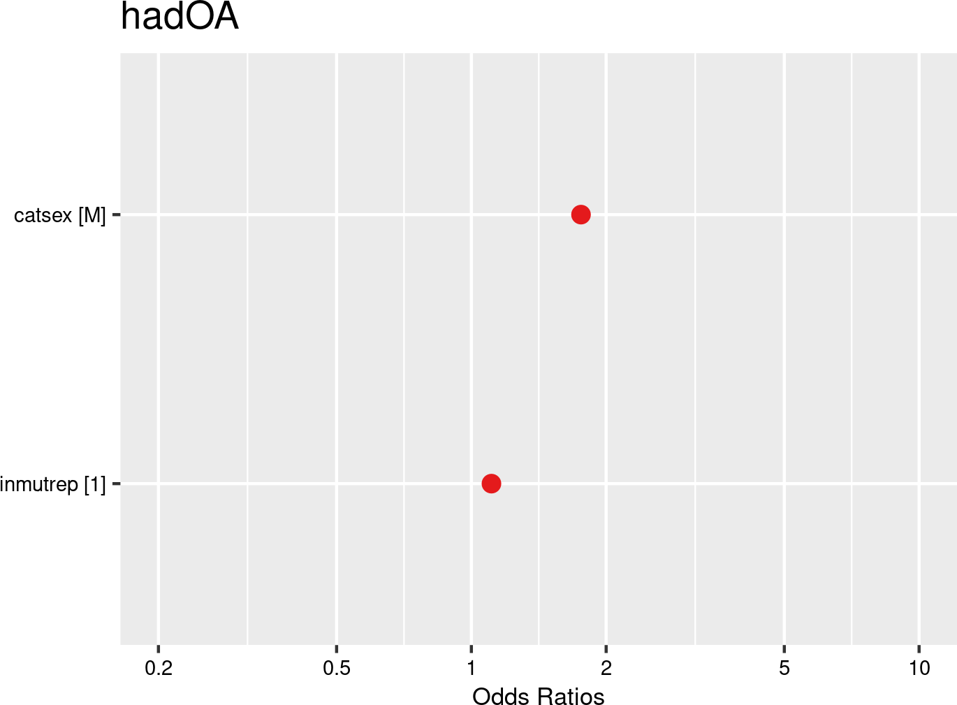
Figure 3.2 shows that workers aged 20-29 (and 30-39) have a 37% (and 14%) higher chance of reporting an OA (both commuting and workplace accidents), while workers aged 60 and above have a 43% lower chance compared to the reference category (under 20), after accounting for significant differences in company representativeness (Section 3.2). The results suggest a trend where older age groups experience lower chance for reporting workplace accidents.
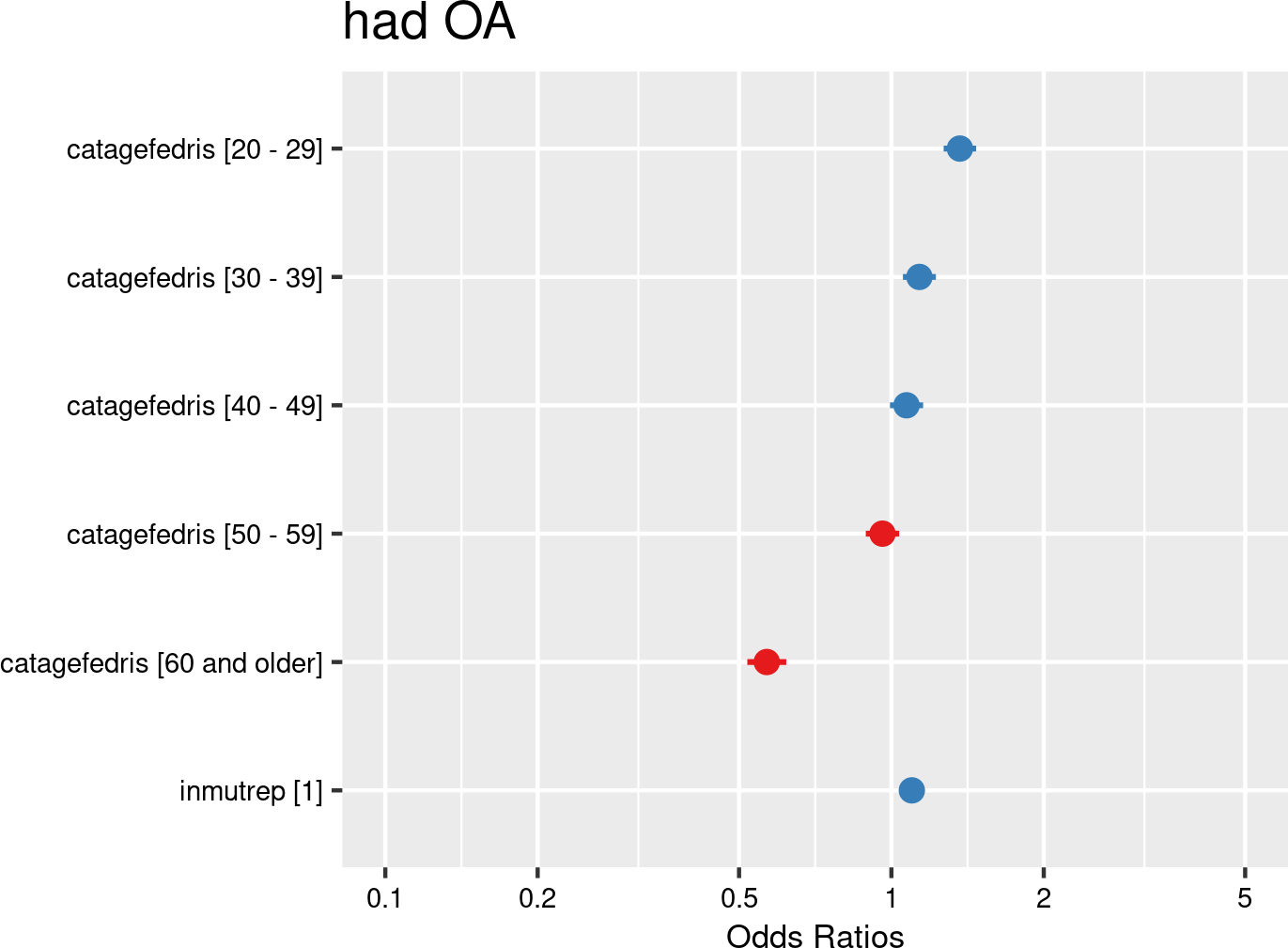

Age categories were introduced as fixed effects, and companies and employees as random effects. The model is based on data from employees with and without OAs from all mutual Liantis ESPP and PS customers. The model is adjusted for representativeness of the company (fixed effect inmutrep) regarding to sector, size and Flemish province.
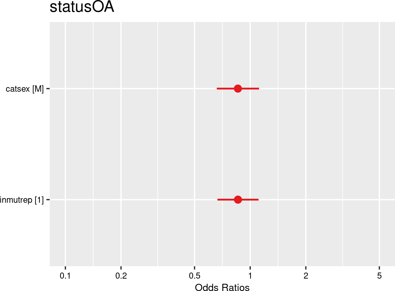
Figure 3.3 shows that age does not significantly determines whether an insurer accepts or rejects an OA claim. This suggests that there is no age-based discrimination in insurance decisions.
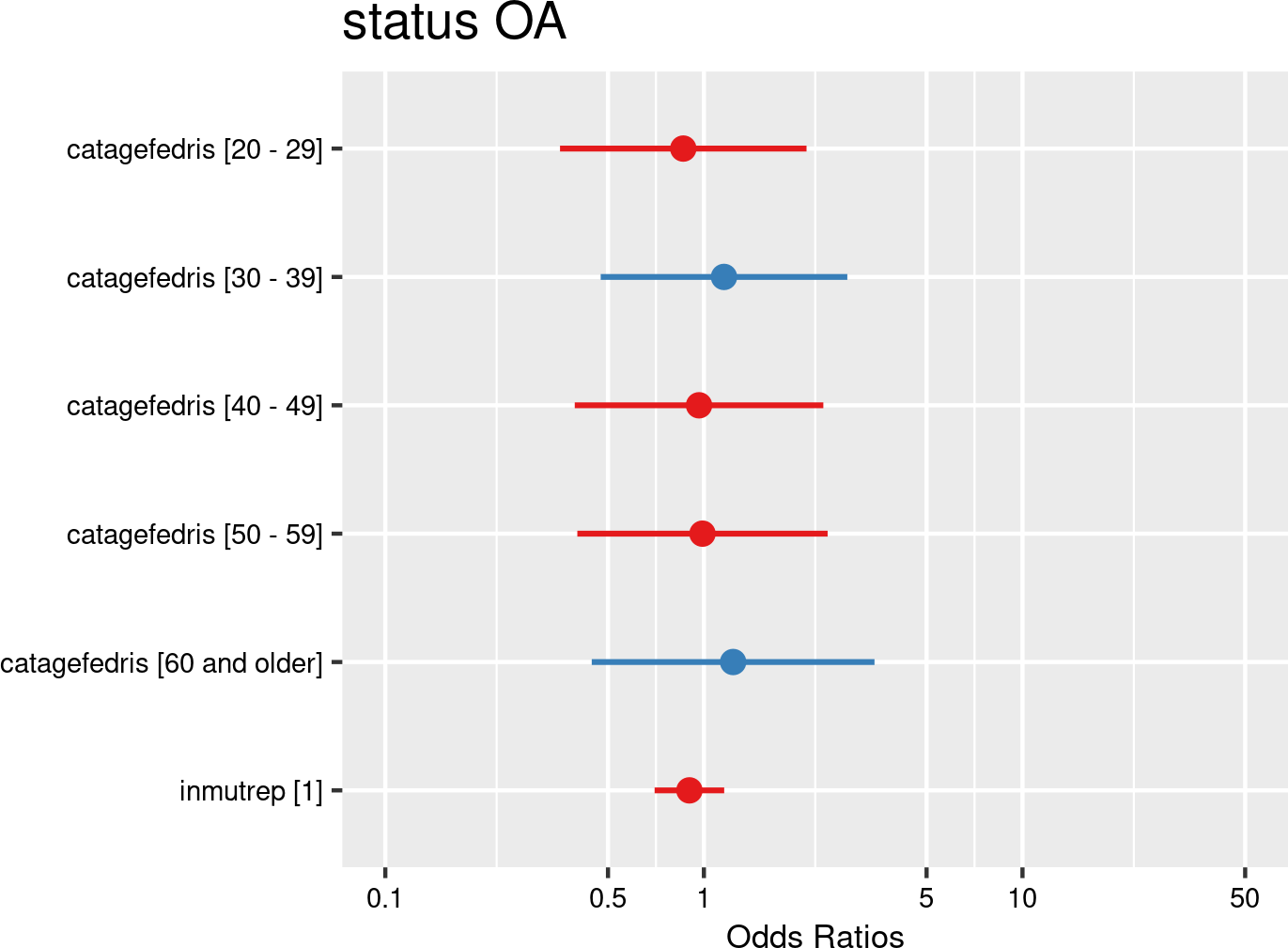

Age categories were introduced as fixed effects, and companies and employees as random effects. The model is based on data from employees notifying OAs from all mutual Liantis ESPP and PS customers. The model is adjusted for representativeness of the company (fixed effect inmutrep) regarding to sector, size and Flemish province.
The results presented in Figure 3.4 do not support earlier findings from literature showing that workers between 45-65 year have a higher incidence of commuting accidents in comparison with the younger workers.
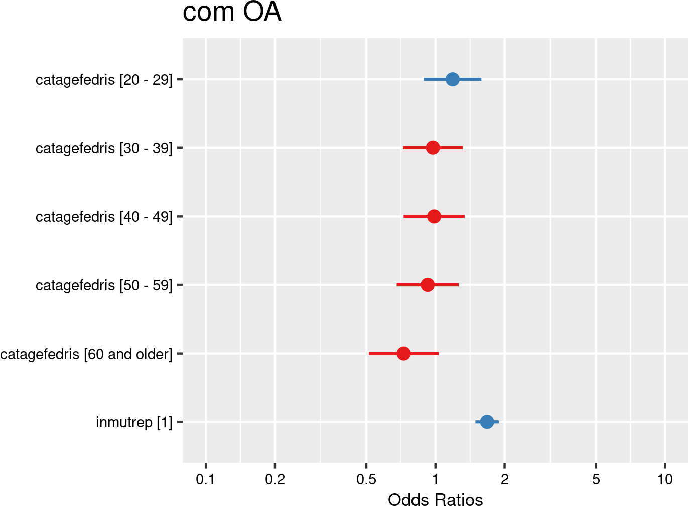

Age categories were introduced as fixed effects, and companies and employees as random effects. The model is based on data from employees with and without OAs from all mutual Liantis ESPP and PS customers. The model is adjusted for representativeness of the company (fixed effect inmutrep) regarding to sector, size and Flemish province.
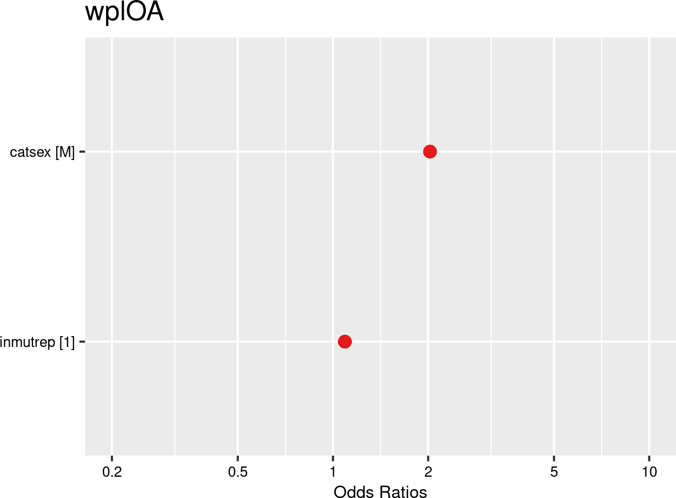
Figure 3.5 shows that workers aged 20-29 have a 47% higher chance of having an accepted workplace accident, while workers aged 60 and above have a 41% lower chance compared to the reference category (under 20). This underscores the findings of several researchers (Yong Jeong (1999), Takahashi & Miura (2016), Kaur et al. (2023)).

Age categories were introduced as fixed effects, and companies and employees as random effects. The model is based on data from employees with and without OAs from all mutual Liantis ESPP and PS customers. The model is adjusted for representativeness of the company (fixed effect inmutrep) regarding to sector, size and Flemish province.
Figure 3.6 (a) and Figure 3.6 (b) present a model estimating the frequency degree of OAs at the company level, in contrast to previous models that focused on individual employee accident probabilities. These figures show that a higher proportion of workers in the age categories 20-29, 30-39, and 40-49 significantly increases the frequency degree of OAs within a company. Conversely, a higher proportion of workers aged 60 and older is associated with a significant decrease in the frequency degree of a company. It is important to note that this trend does not completely align with the relationship between age categories and the likelihood of a workplace OA (where a lower chance of a workplace OA is observed from the age of 30). However, for the calculation of the frequency rate of OAs, accidents without consequences are excluded.
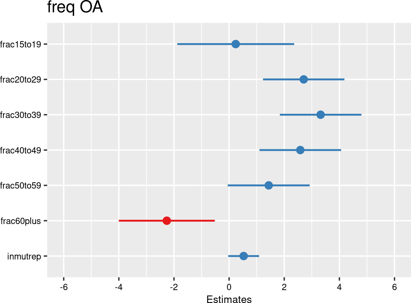

Figure 3.7 (a) and Figure 3.7 (b) present a model estimating the chance for an accepted accident being serious (according to the definition of the Belgian law). These figures indicate that age does not significantly determine whether an workplace OA is classified as serious.
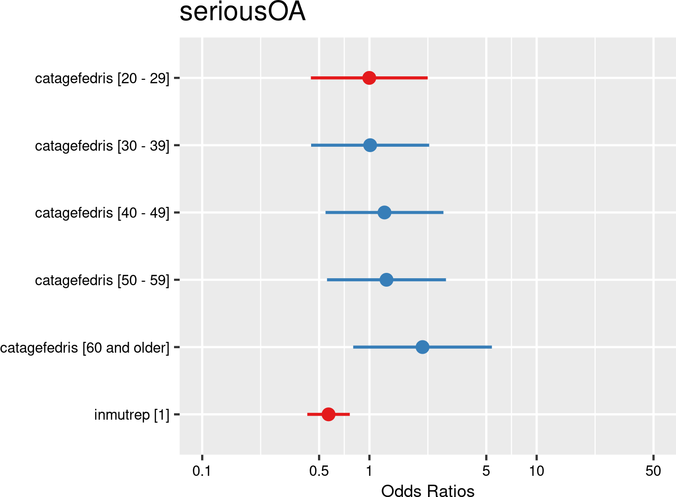

Figure 3.8 (a) and Figure 3.8 (b) are the results of a model assessing the relation between age and the number of absenteeism days. These first 2 figures are based on the absenteeism data provided by FEDRIS (while Figure 3.9 (a) and Figure 3.9 (b) present the same model based on the Liantis PS data). These figures show that age is an important factor in determining the validated number of absenteeism days related to the OA. The number of accepted days off increases significantly with age (e.g., 26% more days for ages 20-29, 88% more days for ages 30-39,…). This aligns with Salminen (2004), which states that older workers experience more severe consequences from OAs.

As mentioned above, Figure 3.9 (a) and Figure 3.9 (b) are the results of the model assessing the relation between age category and number of absenteeism days related to the workplace accident, based on the Liantis PS data. The results are very similar to these of Figure 3.8 above.
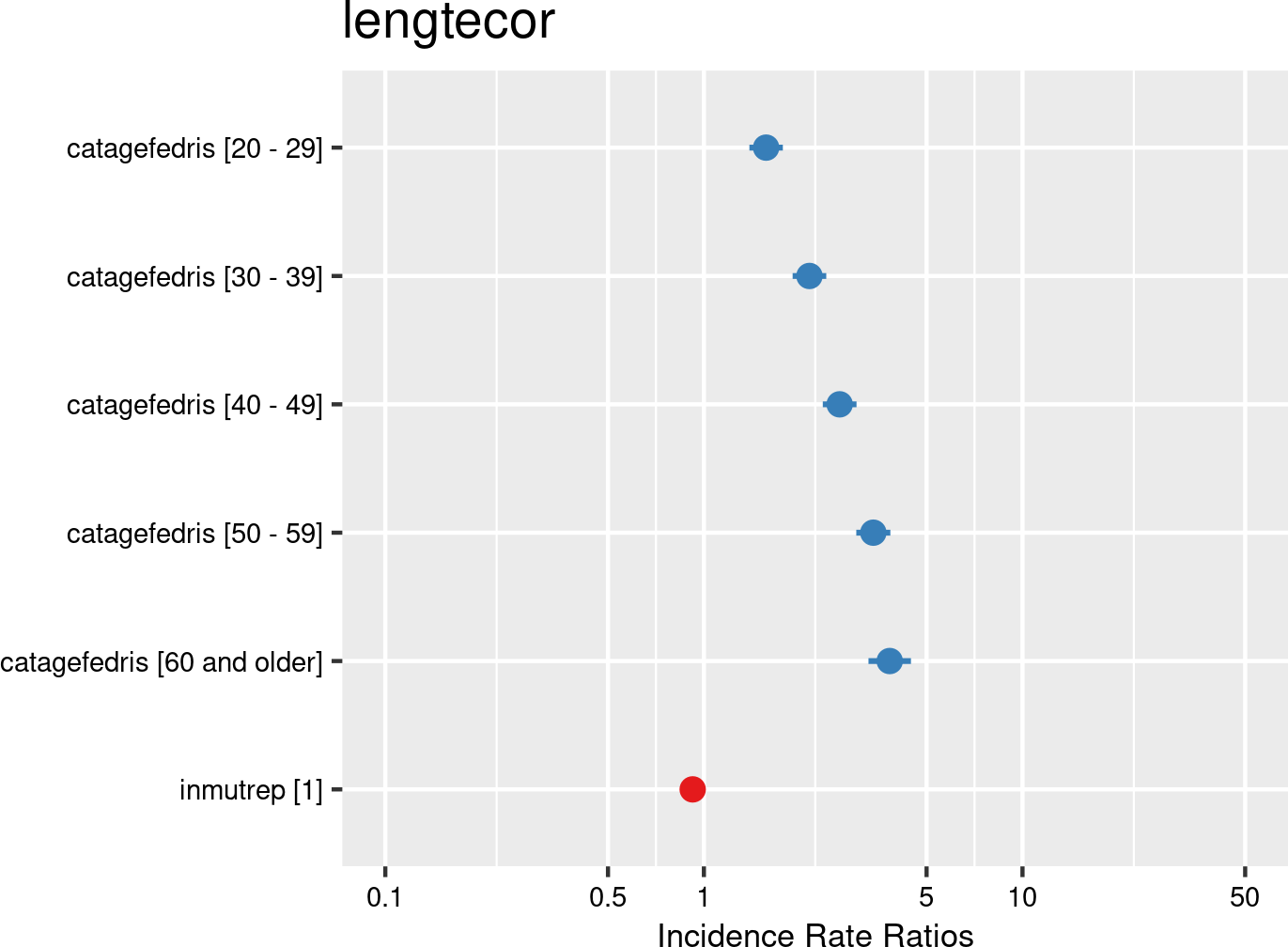

Figure 3.10 (a) and Figure 3.10 (b) show the results of the model that is assessing the relation between age category and direct wage cost of an OA are displayed. It indicates that age seems to be a significant factor in determining the direct wage cost of an OA for an employer. This can be attributed to the higher number of absenteeism days in older age groups, as shown in previous models, as well as the higher wages of older employees.

The next 4 figures (Figure 3.11 (a) and Figure 3.11 (b), Figure 3.12 (a) and Figure 3.12 (b)) are displaying the results of a model assessing the relation between proportion of workers within an age category and the severity degree of a company, which is again a variable at the company level. In the first model (Figure 3.11), the validated number of absenteeism days from FEDRIS was used, while the second model (Figure 3.12) was based on the numbers of days off calculated from the Liantis PS data. These figures show that a higher proportion of workers aged 30-39 and 50-59 significantly increases the severity level within a company.
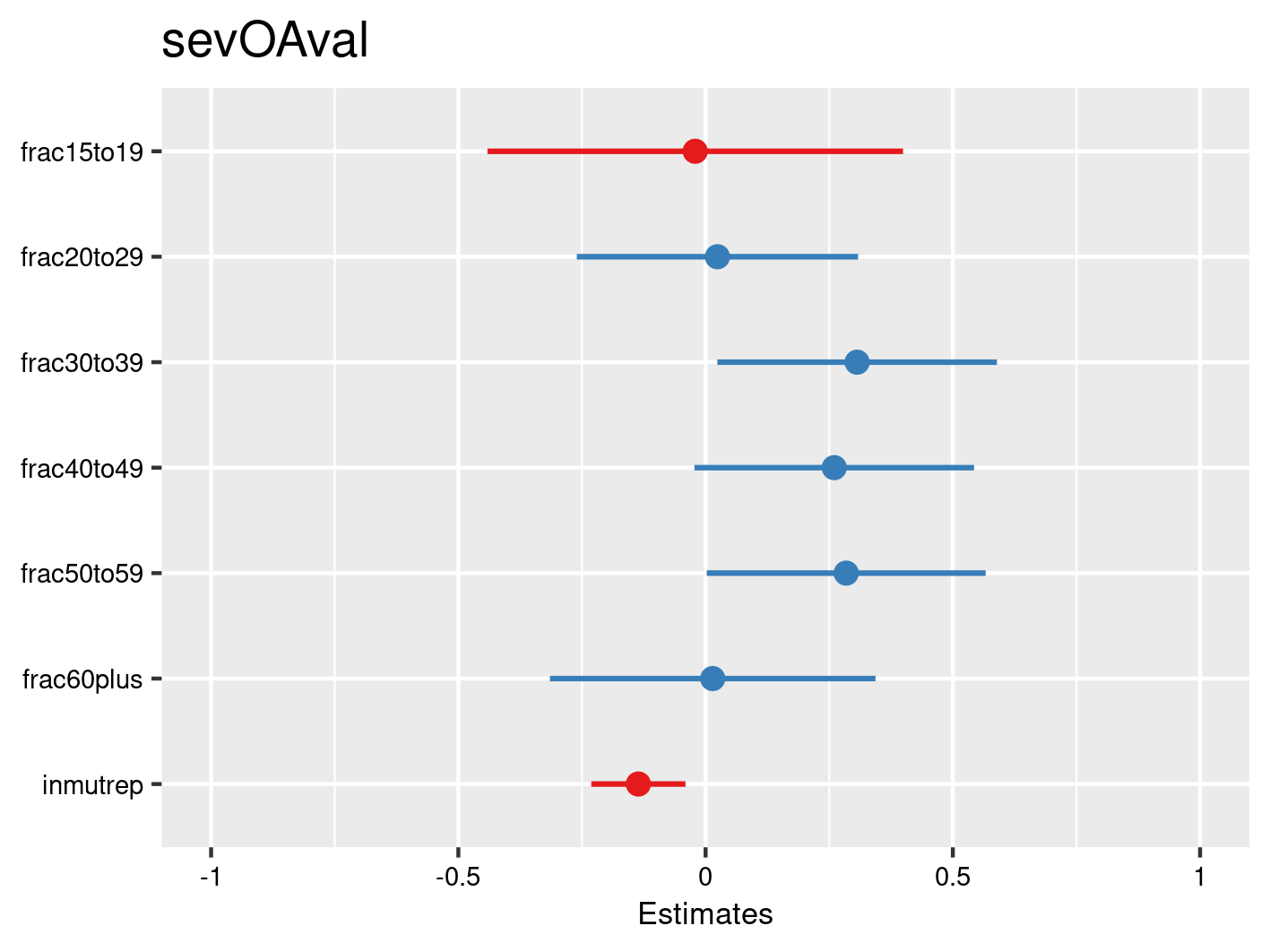

Figure 3.12 shows that a higher proportion of workers aged 30-39 and 40-49 significantly increases the severity level within a company, based on the number of calculated days from Lantis PS data. These results are generally in line with those from the model, which used validated FEDRIS data.

3.4.1.2 Biological sex
3.4.1.2.1 Descriptives
Both NSSO and FEDRIS provide biological sex categories. Liantis PS and ESPP data do contain biological sex variables, but since the FEDRIS notifications do not contain biological age categories, the variable was calculated from the INSZ number (except bis numbers) of the employee. Since sex categories are absent in the notifications, the fit between the derived biological sex of an employee experiencing an OA cannot be compared with the corresponding sex classification in the notification of the accident.
From the tables Table 3.18, Table 3.20 and Table 3.22, some important findings can be noticed. While male workers account for about 50% of the workforce, they account for 60% of all OA notifications. This is a significant overrepresentation.
all accepted occupational accidents
| name | rszall | rszpriv | liaall | fedrisall | totalnot | totalnotmut | totalnotrepmutflan |
|---|---|---|---|---|---|---|---|
| Mannen | 78213055 | 62065095 | 8831706 | 788224 | 126380 | 39103 | 13193 |
| Vrouwen | 74955087 | 52369731 | 8999383 | 439553 | 68405 | 22048 | 12821 |
| name | percrszall | percrszpriv | percliaall | percfedrisall | perctotalnot | perctotalnotmut | perctotalnotrepmutflan |
|---|---|---|---|---|---|---|---|
| Mannen | 51.06 | 54.24 | 49.53 | 64.2 | 64.88 | 63.94 | 50.71 |
| Vrouwen | 48.94 | 45.76 | 50.47 | 35.8 | 35.12 | 36.06 | 49.29 |
commuting accepted occupational accidents
| name | rszall | rszpriv | liaall | fedrisall | totalnot | totalnotmut | totalnotrepmutflan |
|---|---|---|---|---|---|---|---|
| Mannen | 78213055 | 62065095 | 8831706 | 93986 | 12886 | 3596 | 1424 |
| Vrouwen | 74955087 | 52369731 | 8999383 | 107551 | 15482 | 5001 | 2687 |
| name | percrszall | percrszpriv | percliaall | percfedrisall | perctotalnot | perctotalnotmut | perctotalnotrepmutflan |
|---|---|---|---|---|---|---|---|
| Mannen | 51.06 | 54.24 | 49.53 | 46.63 | 45.42 | 41.83 | 34.64 |
| Vrouwen | 48.94 | 45.76 | 50.47 | 53.37 | 54.58 | 58.17 | 65.36 |
workplace accepted occupational accidents
| name | rszall | rszpriv | liaall | fedrisall | totalnot | totalnotmut | totalnotrepmutflan |
|---|---|---|---|---|---|---|---|
| Mannen | 78213055 | 62065095 | 8831706 | 761309 | 113494 | 35507 | 11769 |
| Vrouwen | 74955087 | 52369731 | 8999383 | 365728 | 52923 | 17047 | 10134 |
| name | percrszall | percrszpriv | percliaall | percfedrisall | perctotalnot | perctotalnotmut | perctotalnotrepmutflan |
|---|---|---|---|---|---|---|---|
| Mannen | 51.06 | 54.24 | 49.53 | 67.55 | 68.2 | 67.56 | 53.73 |
| Vrouwen | 48.94 | 45.76 | 50.47 | 32.45 | 31.8 | 32.44 | 46.27 |
3.4.1.2.2 Models
The following Table 3.23 summarizes the results of the models assessing the relationship between biological sex (Female or Male) and the nine outcomes. Below the table, you can find the data on which each model is based. The results of the nine models are then presented both graphically and in a table.
| catsex | chance to notify | chance on refusal | chance commuting | chance workplace | freq degree | chance serious | nDays TAO V/C | cost | sev degree V/C |
|---|---|---|---|---|---|---|---|---|---|
| Female | REF | REF | REF | REF | < | REF | REF | REF | ns |
| Male | > | ns | < | > | > | > | ns/> | > | >/> |
| occur | accept | occur | occur | occur | severe | severe | severe | severe | |
| empl | empl | empl | empl | comp | empl | empl | empl | comp | |
| c/w all | c/w ref | c acc | w acc | w acc | w acc | w acc | w acc | w acc |
- occur: data include all workers, chance for occurrence is calculated for the outcome
- accept: data include only workers with a notification of OA
- severe: data include only workers with an accepted OA
- c/w all: commuting and workplace accidents, including refused and accidents without decisions
- c/w ref: accepted or refused commuting and workplace accidents
- c acc: accepted commuting accidents
- w acc: accepted workplace accidents
- empl: the outcome is situated at the individual level
- comp: the outcome is situated at the company level
- nDaysTAO: number of days absenteeism related to the OA
- V/C: Validated number of days (available from FEDRIS) / Calculated number of days (based on the Liantis PS data)
Biological sex and occupational accidents
- We notice a higher occupational accident chance for males. This is only noticed for accepted workplace occupational accidents and not for accepted commuting accidents.
- There was no relation between biological sex and the chance for an occupational accident to be categorized as severe.
- If a company has a higher proportion of male workers, it may have a higher frequency degree and severity degree of occupational accidents.
- The number of days off and the wage cost related to an occupational accident is significantly higher for male workers.
From Figure 3.13 (a) and Figure 3.13 (b) we learn that workers in the category male have a 76% higher chance to notify an OA (both commuting and workplace accidents) than the female reference category (after accounting for significant differences in representativeness of the company).

Biological sex categories were introduced as fixed effects, and companies and employees as random effects. The model is based on data from employees with and without OAs from all mutual Liantis ESPP and PS customers. The model is adjusted for representativeness of the company (fixed effect inmutrep) regarding to sector, size and Flemish province.
From Figure 3.14 (a) and Figure 3.14 (b) we learn that sex does not not seem to be an important determinant for acceptance or refusal of an OA by an insurer.

Biological sex categories were introduced as fixed effects, and companies and employees as random effects. The model is based on data from employees notifying OAs from all mutual Liantis ESPP and PS customers. The model is adjusted for representativeness of the company (fixed effect inmutrep) regarding to sector, size and Flemish province.
From Figure 3.15 (a) and Figure 3.15 (b) we learn that the effect of biological sex is significant in the current study. Also the direction of the observed lower chance for males is consistent with literature which does state that women are at higher risk for occupational commuting accidents (Craig et al., 2023; Federal Public Service Health, Food Chain Safety and Environment, 2022; López et al., 2017; Salerno & Giliberti, 2019, 2021).

Biological sex categories were introduced as fixed effects, and companies and employees as random effects. The model is based on data from employees with and without OAs from all mutual Liantis ESPP and PS customers. The model is adjusted for representativeness of the company (fixed effect inmutrep) regarding to sector, size and Flemish province.
From Figure 3.16 (a) and Figure 3.16 (b) we learn that male workers have a 103% higher chance on an accepted workplace accident than female workers (after accounting for significant differences in representativeness of the company). This is in line with previous findings (Feijó et al., 2018; Hendricks et al., 2024; Neves & Fonseca, 2023).

Biological sex categories were introduced as fixed effects, and companies and employees as random effects. The model is based on data from employees with and without OAs from all mutual Liantis ESPP and PS customers. The model is adjusted for representativeness of the company (fixed effect inmutrep) regarding to sector, size and Flemish province.
From Figure 3.17 (a) and Figure 3.17 (b) we learn that the proportion of male workers has a significant increasing effect on the frequency degree of a company, while the proportion of female workers has a significant decreasing effect on the frequency degree of a company. Even if a higher proportion of male workers in a company is generally associated with a higher chance of OAs, we would not expect this to be attributed to gender ratio alone, but rather due to the types of jobs men and women typically perform. The specific risk would also depend on job roles, industry, and organisational factors, not just gender ratio alone.
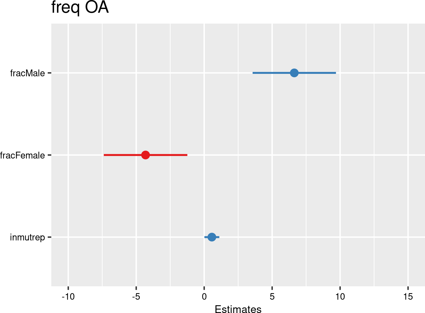

Biological sex category proportions were introduced as fixed effects, and companies as random effects. The model is based on data of all mutual Liantis ESPP and PS customers. The model is adjusted for representativeness of the company (fixed effect inmutrep) regarding to sector, size and Flemish province.
From Figure 3.18 (a) and Figure 3.18 (b) we learn that sex does seem to be an important determinant for classifying an workplace OA as serious: men tend to have a 89% higher chance on a serious accident.
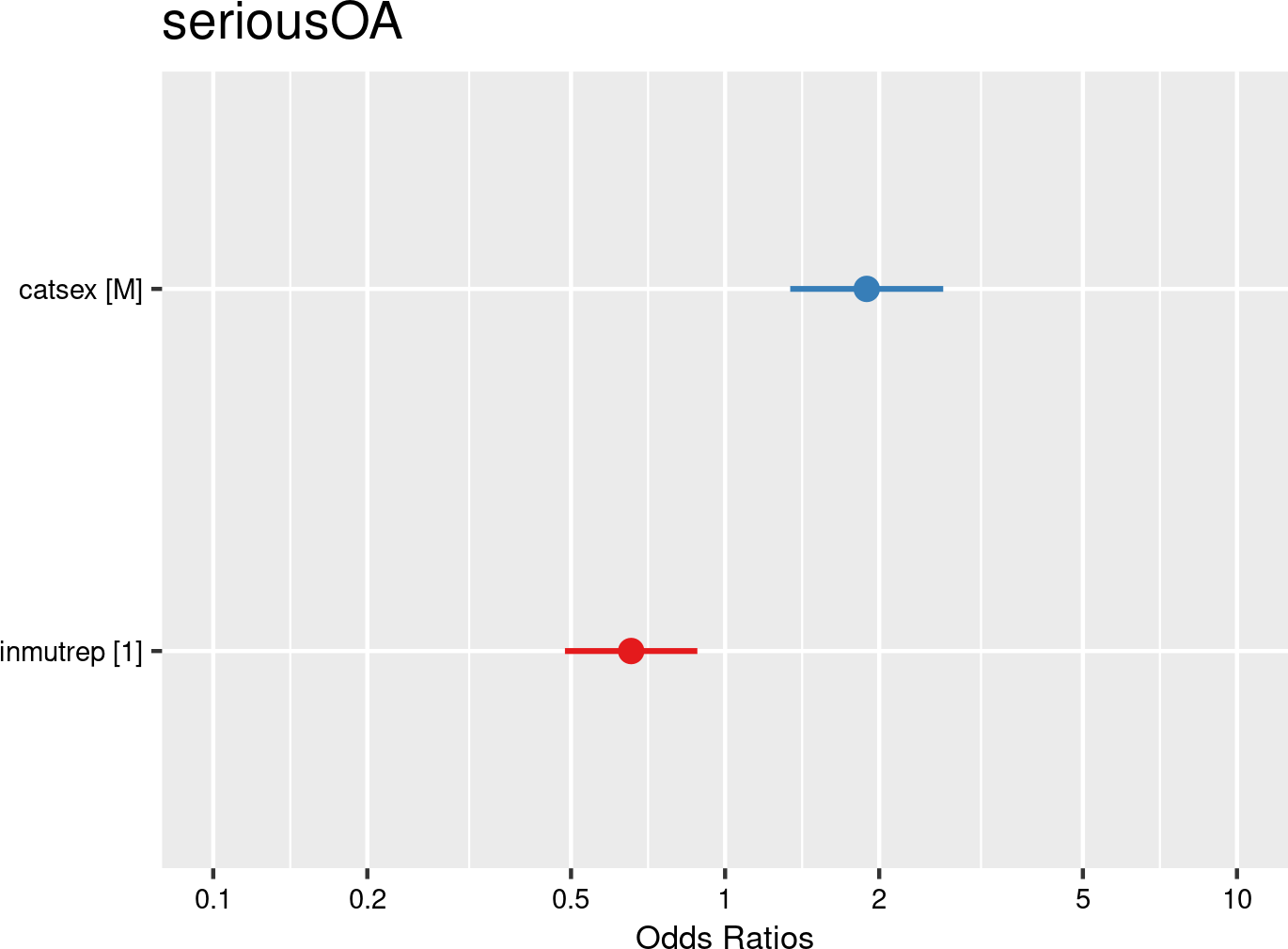

Biological sex categories were introduced as fixed effects, and companies and employees as random effects. The model is based on data of all mutual Liantis ESPP and PS customers. The model is adjusted for representativeness of the company (fixed effect inmutrep) regarding to sector, size and Flemish province.
Figure 3.19 (a) and Figure 3.19 (b) indicate that biological sex does not appear to be a significant determinant of the validated number of days of work unavailability. This aligns with the broader literature, which reports inconsistent findings regarding the role of sex in recovery duration. In our study, the number of accepted days of absence does not differ significantly between men and women, suggesting that men do not experience longer absences due to workplace accidents, in contrary to the findings of the Medex study (Federal Public Service Health, Food Chain Safety and Environment, 2022). Our results also diverge from those of Fontaneda et al. (2019), who reported longer absences among women. Even if women tend to have longer recovery periods following OAs, particularly in lower-responsibility or female-dominated roles, this pattern likely varies depending on occupation, job responsibilities, and workplace context.
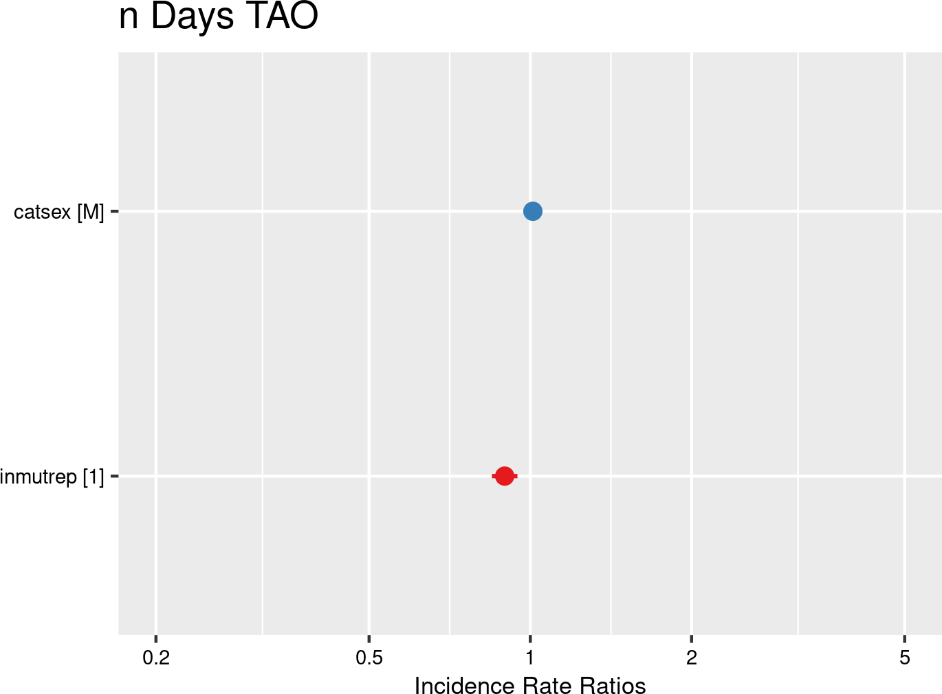

Biological sex categories were introduced as fixed effects, and companies and employees as random effects. The model is based on data of all mutual Liantis ESPP and PS customers. The model is adjusted for representativeness of the company (fixed effect inmutrep) regarding to sector, size and Flemish province.
From Figure 3.20 (a) and Figure 3.20 (b) we learn that sex seems to be a determinant for the calculated number of days of unavailability for work from Liantis PS data. The number of calculated days increases significantly for male workers compared to female workers. The results diverge from the results of model6, where validated FEDRIS data are used.
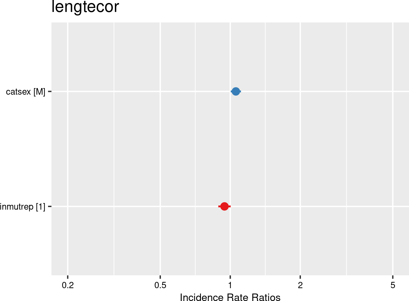

Biological sex categories were introduced as fixed effects, and companies and employees as random effects. The model is based on data of all mutual Liantis ESPP and PS customers. The model is adjusted for representativeness of the company (fixed effect inmutrep) regarding to sector, size and Flemish province.
From Figure 3.21 (a) and Figure 3.21 (b) we learn that sex does seem to be an significant determinant for the direct wage cost of an OA for an employer: the cost for male workers is significantly higher. Higher costs for men may seem plausible since they are more likely to work in higher-wage, higher-risk jobs and receive greater wage compensation for risk. This pattern is reinforced by occupational segregation and wage structures across industries.
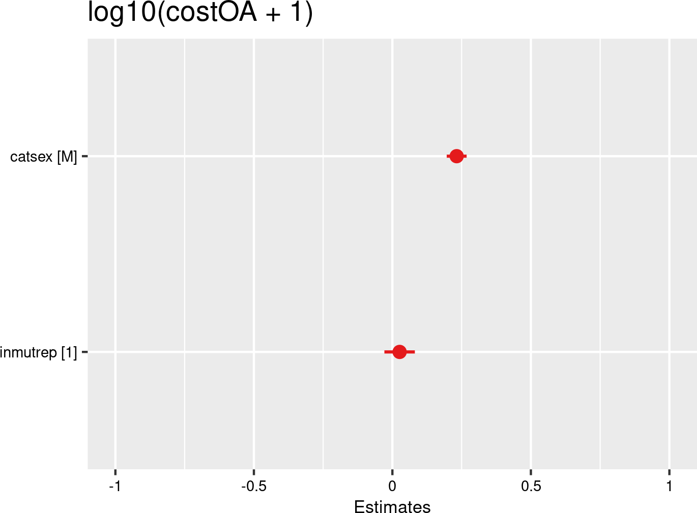

Biological sex categories were introduced as fixed effects, and companies and employees as random effects. The model is based on data of all mutual Liantis ESPP and PS customers. The model is adjusted for representativeness of the company (fixed effect inmutrep) regarding to sector, size and Flemish province.
From Figure 3.22 (a) and Figure 3.22 (b) we learn that the proportion of male workers has a signicant increasing effect on the severity degree of a company.
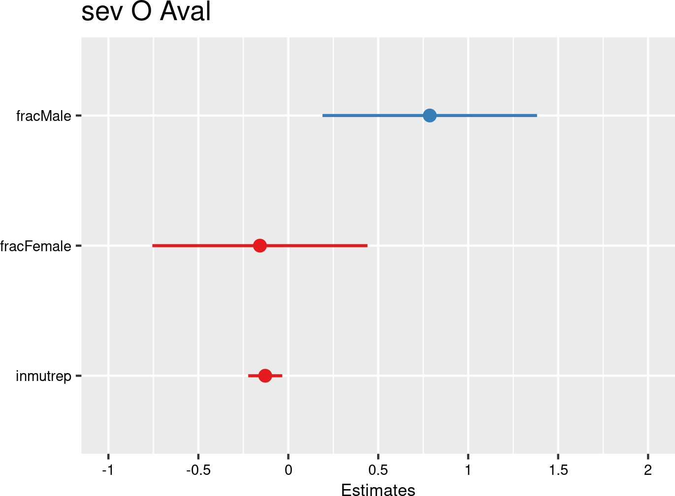

Biological sex category proportions were introduced as fixed effects, and companies as random effects. The model is based on data of all mutual Liantis ESPP and PS customers. The model is adjusted for representativeness of the company (fixed effect inmutrep) regarding to sector, size and Flemish province.
From Figure 3.23 (a) and Figure 3.23 (b) we learn that the proportion of male workers has a signicant increasing effect on the severity degree of a company using the number of calculated days from Liantis PS data. The results are equivalent to the results of model8 where validated FEDRIS data are used.
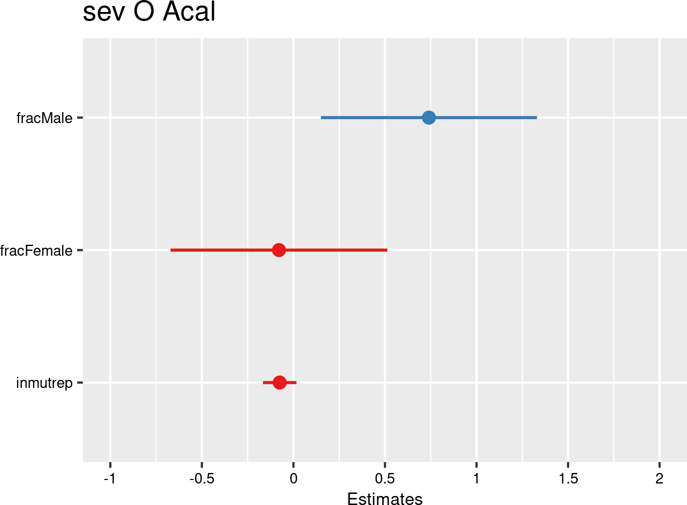

Biological sex category proportions were introduced as fixed effects, and companies as random effects. The model is based on data of all mutual Liantis ESPP and PS customers. The model is adjusted for representativeness of the company (fixed effect inmutrep) regarding to sector, size and Flemish province.
3.4.1.3 Work experience (seniority with the employer)
3.4.1.3.1 Descriptives
Literature generally indicates a correlation between limited work experience and a higher incidence of OA. However, since work experience data is often unavailable, seniority (the number of years an employee has worked with a specific employer) is used as a proxy.
Unfortunately, NSSO does not provide data on seniority with the employer, but FEDRIS does. Liantis PS data includes the start and end dates of an employee’s contracts with a specific employer. So, the proxy for experience was derived by calculating the difference between the last day of the last contract and the first day of the first contract with the same employer. This time difference was categorized using the same categories as in the FEDRIS reports and notifications.
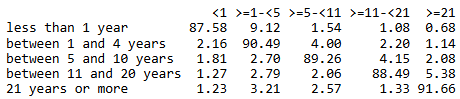
Since seniority categories are included in the notifications, the calculated seniority of an employee involved in an OA can be compared with the corresponding seniority classification in the accident notification. The results of this comparison are displayed in Figure 3.24. The correlation between the two datasets is 0.85, which indicates a strong positive relationship. This suggests that the seniority categories derived from Liantis PS data align well with those in FEDRIS data, making them both suitable for further analysis.
In the next 6 tables, an overview of all (accepted) OAs (Table 3.24 and Table 3.25), the commuting OAs (Table 3.26 and Table 3.27) and the workplace OAs (Table 3.28 and Table 3.29) are given. In the first table ((Table 3.24, Table 3.26 and Table 3.28), the absolute numbers are provided stratified per experience category, next to the total number of employees, as available in the Liantis PS database. As mentioned above, the NSSO does not provide information about seniority. In the second table (Table 3.25, Table 3.27 and Table 3.29), the relative numbers of the OAs per seniority category are provided as percentages.
From the tables Table 3.25, Table 3.27 and Table 3.29, some important findings can be noticed. While workers with a seniority less than 1 year account for >33% of employees within liantis customers, they account for <33% of OA notifications.
all accepted occupational accidents
| catexp | rszall | rszpriv | liaall | fedrisall | totalnot | totalnotmut | totalnotrepmutflan |
|---|---|---|---|---|---|---|---|
| less than 1 year | NA | NA | 6337684 | 389735 | 41605 | 15470 | 5970 |
| between 1 and 4 years | NA | NA | 5389165 | 361530 | 57288 | 18908 | 7366 |
| between 5 and 10 years | NA | NA | 3252844 | 210007 | 33513 | 9779 | 4057 |
| between 11 and 20 years | NA | NA | 2120661 | 155635 | 25239 | 6135 | 2869 |
| 21 years or more | NA | NA | 955512 | 97582 | 16228 | 3119 | 1704 |
| unknown | NA | NA | NA | 138888 | 21346 | 7824 | 4064 |
| catexp | percrszall | percrszpriv | percliaall | percfedrisall | perctotalnot | perctotalnotmut | perctotalnotrepmutflan |
|---|---|---|---|---|---|---|---|
| less than 1 year | NA | NA | 35.1 | 32.1 | 23.9 | 29.0 | 27.2 |
| between 1 and 4 years | NA | NA | 29.8 | 29.8 | 32.9 | 35.4 | 33.5 |
| between 5 and 10 years | NA | NA | 18.0 | 17.3 | 19.3 | 18.3 | 18.5 |
| between 11 and 20 years | NA | NA | 11.7 | 12.8 | 14.5 | 11.5 | 13.1 |
| 21 years or more | NA | NA | 5.3 | 8.0 | 9.3 | 5.8 | 7.8 |
| unknown | NA | NA | NA | NA | NA | NA | NA |
commuting accepted occupational accidents
| catexp | rszall | rszpriv | liaall | fedrisall | totalnot | totalnotmut | totalnotrepmutflan |
|---|---|---|---|---|---|---|---|
| less than 1 year | NA | NA | 6337684 | 62403 | 6319 | 2438 | 1093 |
| between 1 and 4 years | NA | NA | 5389165 | 60578 | 7820 | 2530 | 1159 |
| between 5 and 10 years | NA | NA | 3252844 | 35759 | 4680 | 1244 | 590 |
| between 11 and 20 years | NA | NA | 2120661 | 28140 | 3859 | 874 | 442 |
| 21 years or more | NA | NA | 955512 | 20404 | 3036 | 537 | 319 |
| unknown | NA | NA | NA | 19026 | 2673 | 976 | 509 |
| catexp | percrszall | percrszpriv | percliaall | percfedrisall | perctotalnot | perctotalnotmut | perctotalnotrepmutflan |
|---|---|---|---|---|---|---|---|
| less than 1 year | NA | NA | 35.1 | 30.1 | 24.6 | 32.0 | 30.3 |
| between 1 and 4 years | NA | NA | 29.8 | 29.2 | 30.4 | 33.2 | 32.2 |
| between 5 and 10 years | NA | NA | 18.0 | 17.3 | 18.2 | 16.3 | 16.4 |
| between 11 and 20 years | NA | NA | 11.7 | 13.6 | 15.0 | 11.5 | 12.3 |
| 21 years or more | NA | NA | 5.3 | 9.8 | 11.8 | 7.0 | 8.9 |
| unknown | NA | NA | NA | NA | NA | NA | NA |
workplace accepted occupational accidents
| catexp | rszall | rszpriv | liaall | fedrisall | totalnot | totalnotmut | totalnotrepmutflan |
|---|---|---|---|---|---|---|---|
| less than 1 year | NA | NA | 6337684 | 327332 | 35286 | 13032 | 4877 |
| between 1 and 4 years | NA | NA | 5389165 | 300952 | 49468 | 16378 | 6207 |
| between 5 and 10 years | NA | NA | 3252844 | 174248 | 28833 | 8535 | 3467 |
| between 11 and 20 years | NA | NA | 2120661 | 127495 | 21380 | 5261 | 2427 |
| 21 years or more | NA | NA | 955512 | 77178 | 13192 | 2582 | 1385 |
| unknown | NA | NA | NA | 119862 | 18673 | 6848 | 3555 |
| catexp | percrszall | percrszpriv | percliaall | percfedrisall | perctotalnot | perctotalnotmut | perctotalnotrepmutflan |
|---|---|---|---|---|---|---|---|
| less than 1 year | NA | NA | 35.1 | 32.5 | 23.8 | 28.5 | 26.6 |
| between 1 and 4 years | NA | NA | 29.8 | 29.9 | 33.4 | 35.8 | 33.8 |
| between 5 and 10 years | NA | NA | 18.0 | 17.3 | 19.5 | 18.6 | 18.9 |
| between 11 and 20 years | NA | NA | 11.7 | 12.7 | 14.4 | 11.5 | 13.2 |
| 21 years or more | NA | NA | 5.3 | 7.7 | 8.9 | 5.6 | 7.5 |
| unknown | NA | NA | NA | NA | NA | NA | NA |
3.4.1.3.2 Models
The following Table 3.30 summarizes the results of the models assessing the relationship between work experience categories (seniority with the employer) and the nine outcomes. Below the table, you can find the data on which each model is based. The results of the nine models are then presented both graphically and in a table.
| catsen | chance to notify | chance on refusal | chance commuting | chance workplace | freq degree | chance serious | nDays TAO V/C | cost | sev degree V/C |
|---|---|---|---|---|---|---|---|---|---|
| less than 1 | REF | REF | REF | REF | < | REF | REF | REF | ns/< |
| 1 to 4 | ns | ns | < | ns | ns | > | >/> | > | ns |
| 5 to 10 | < | ns | < | < | ns | > | >/> | > | ns |
| 11 to 20 | < | ns | ns | < | ns | ns | >/> | > | ns |
| 21 and more | < | ns | < | < | ns | ns | >/> | > | ns |
| occur | accept | occur | occur | occur | severe | severe | severe | severe | |
| empl | empl | empl | empl | comp | empl | empl | empl | comp | |
| c/w all | c/w ref | c acc | w acc | w acc | w acc | w acc | w acc | w acc |
- occur: data include all workers, chance for occurrence is calculated for the outcome
- accept: data include only workers with a notification of OA
- severe: data include only workers with an accepted OA
- c/w all: commuting and workplace accidents, including refused and accidents without decisions
- c/w ref: accepted or refused commuting and workplace accidents
- c acc: accepted commuting accidents
- w acc: accepted workplace accidents
- empl: the outcome is situated at the individual level
- comp: the outcome is situated at the company level
- nDaysTAO: number of days absenteeism related to the OA
- V/C: Validated number of days (available from FEDRIS) / Calculated number of days (based on the Liantis PS data)
Work experience (seniority with the employer) and occupational accidents
- We notice a trend of lower occupational accident chances with higher seniority. This is only noticed for workplace occupational accidents and not for commuting accidents.
- There was some evidence that workers in the categories 1-4 and 5-10 years of seniority have a higher chance for an occupational accident to be categorized as serious.
- If a company has a higher proportion of workers with less than 1 year seniority, it may have a lower frequency degree of occupational accidents.
- The number of days off and the wage cost related to an occupational accident increases significantly with seniority.
Figure 3.25 (a) and Figure 3.25 (b) shows that workers in with 1-4 years seniority do not have a lower chance of reporting an OA (both commuting and workplace accidents). Workers with higher seniority although do have a lower chance (12% to 39%) compared to the reference category <1 year (after accounting for significant differences in company representativeness). Although research is inconsistent, also previous studies generally report a trend of lower OA rates with increased experience (Breslin, 2006; Jeong, 2021; Morassaei et al., 2012).
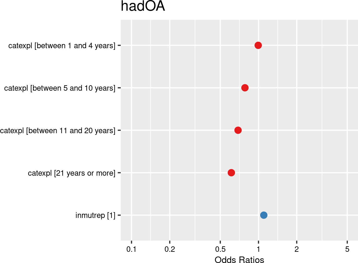

Work experience categories were introduced as fixed effects, and companies and employees as random effects. The model is based on data from employees with and without OAs from all mutual Liantis ESPP and PS customers. The model is adjusted for representativeness of the company (fixed effect inmutrep) regarding to sector, size and Flemish province.
From Figure 3.26 (a) and Figure 3.26 (b), it can be concluded that seniority does not not seem to be an important determinant for acceptance or refusal of an OA by an insurer. This is in line with expectations: we do not expect that based on seniority an OA would be accepted or refused.
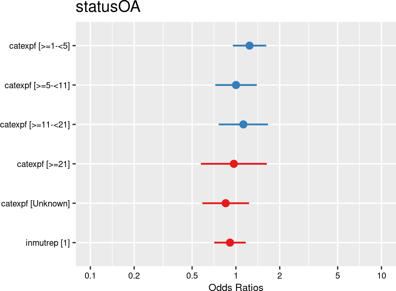

Work experience categories were introduced as fixed effects, and companies and employees as random effects. The model is based on data from employees notifying OAs from all mutual Liantis ESPP and PS customers. The model is adjusted for representativeness of the company (fixed effect inmutrep) regarding to sector, size and Flemish province.
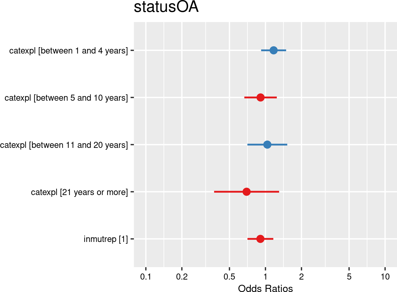

Work experience categories were introduced as fixed effects, and companies and employees as random effects. The model is based on data from employees notifying OAs from all mutual Liantis ESPP and PS customers. The model is adjusted for representativeness of the company (fixed effect inmutrep) regarding to sector, size and Flemish province.
According to Figure 3.28 (a) and Figure 3.28 (b), seniority does not appear to be a significant factor in determining the likelihood of an accepted commuting accident.


Work experience categories were introduced as fixed effects, and companies and employees as random effects. The model is based on data from employees with and without OAs from all mutual Liantis ESPP and PS customers. The model is adjusted for representativeness of the company (fixed effect inmutrep) regarding to sector, size and Flemish province.
Figure 3.29 (a) and Figure 3.29 (b) demonstrate that workers with more seniority (in categories 5-10 and higher) have a 19% to 36% lower chance (after accounting for significant differences in representativeness of the company) on workplace OA. This is in line with a number of former studies, reporting a lower chance for OAs with higher experience (Breslin, 2006; Jeong, 2021; Morassaei et al., 2012).
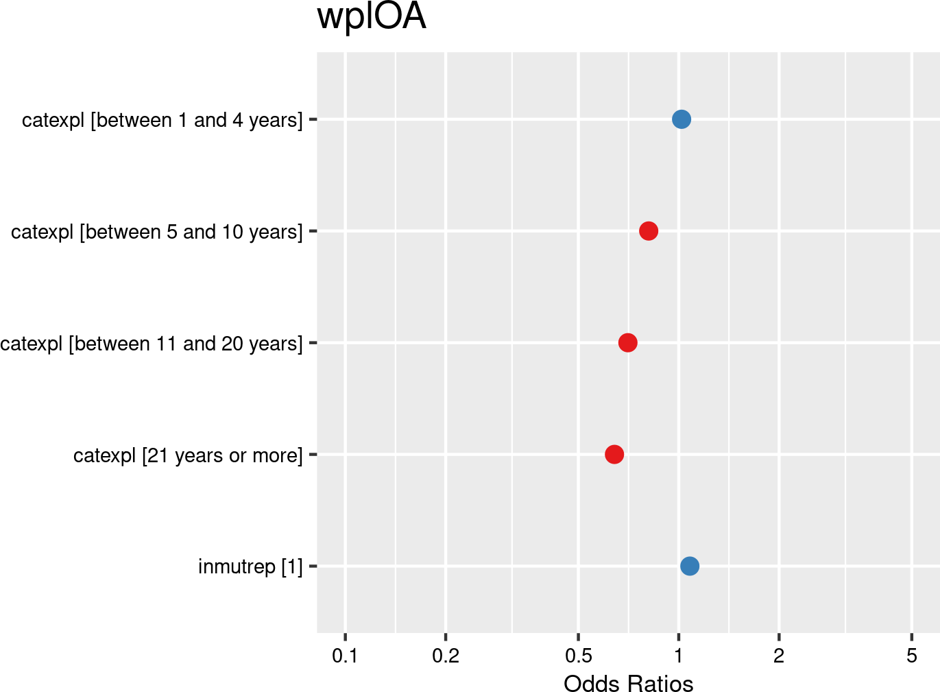

Work experience categories were introduced as fixed effects, and companies and employees as random effects. The model is based on data from employees with and without OAs from all mutual Liantis ESPP and PS customers. The model is adjusted for representativeness of the company (fixed effect inmutrep) regarding to sector, size and Flemish province.
Figure 3.30 (a) and Figure 3.30 (b) show that the proportion of workers in the categories <1 year has a significant decreasing effect on the frequency degree of a company. At first sight, this in contrast with expectations. Possible explanations may lie in how both the outcome and the independent variable are operationalized. For calculating the frequency degree, OAs without consequences are excluded. Since younger (and generally less experienced) workers are known to have a higher incidence of OA, but less severe ones, this may partly explain the findings. Another explanation could be the use of the concept of ‘proportion,’ which indirectly considers the size of the company. In a large company, the same number of workers in this category will result in a much lower proportion compared to a small company. A third explanation could be the inconsistency in literature regarding this relationship; since some studies did not find support for this relation between work experience and OA incidence (Monteiro Ferreira et al., 2020).
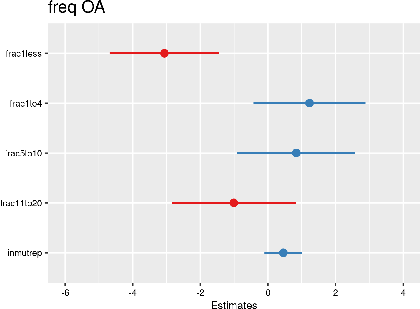

Work experience category proportions were introduced as fixed effects, and companies as random effects. The model is based on data of all mutual Liantis ESPP and PS customers. The model is adjusted for representativeness of the company (fixed effect inmutrep) regarding to sector, size and Flemish province.
Figure 3.31 (a) and Figure 3.31 (b) show that work experience seems to be a determinant for classifying a workplace OA as serious, at least for workers with up to ten years of work experience. This is partially in line with findings of Yedla et al. (2020), who suggests that job experience is an important variable to predict the seriousness of an injury. We should keep in mind that the definition of a serious workplace accident in Belgium may have played a role since not every OA with injury is classified as serious. Moreover, there exist also methodological differences with existing literature: we modelled the likelihood of an OA being categorized as serious, whereas previous research mostly focused on the likelihood of an individual worker experiencing a serious accident.
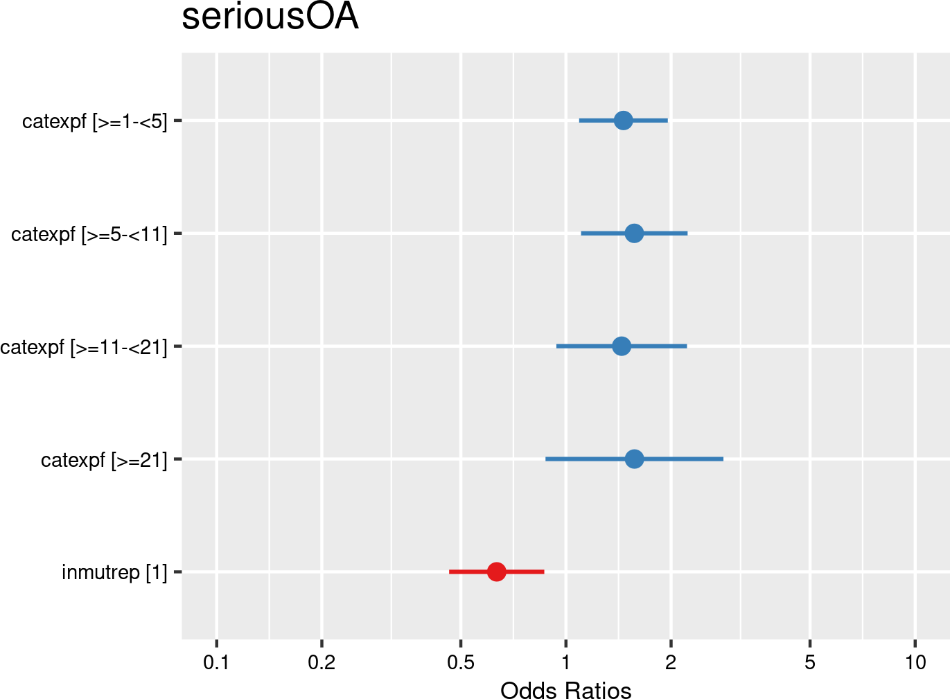

Work experience categories were introduced as fixed effects, and companies and employees as random effects. The model is based on data of all mutual Liantis ESPP and PS customers. The model is adjusted for representativeness of the company (fixed effect inmutrep) regarding to sector, size and Flemish province.
Figure 3.32 (a) and Figure 3.32 (b) are the results of a model assessing the relation between seniority and the number of absenteeism days. These first 2 figures are based on the absenteeism data provided by FEDRIS (while Figure 3.33 (a) and Figure 3.33 (b) present the same model based on the Liantis PS data). These figures show that work seniority is an important factor in determining the validated number of absenteeism days related to the OA.
According to Figure 3.32 (a) and Figure 3.32 (b), the number of accepted days increases significantly with seniority category by 6-9%.
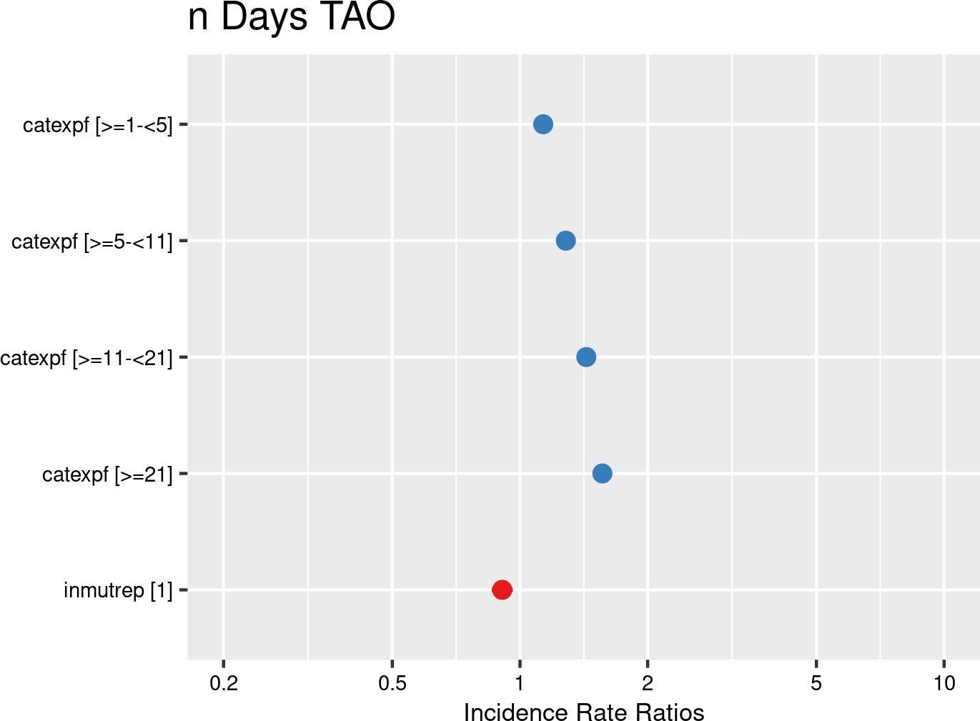

Work experience categories were introduced as fixed effects, and companies and employees as random effects. The model is based on data of all mutual Liantis ESPP and PS customers. The model is adjusted for representativeness of the company (fixed effect inmutrep) regarding to sector, size and Flemish province.
According to Figure 3.33 (a) and Figure 3.33 (b), which present the model results estimating the relationship between seniority category and the calculated number of absenteeism days based on Liantis PS data, the number of absenteeism days increases significantly with seniority, ranging from 19% to 80%.
The observed trend -where a higher seniority corresponds to more days lost from work- aligns with previous research findings (Margolis, 2010; Yedla et al., 2020). Additionally, the slightly larger effect size found in calculations using the Liantis PS data compared to the FEDRIS absenteeism data might be due to the Liantis PS dataset being considerably smaller, with fewer than half the number of employers and less than one-fifth the number of employees.
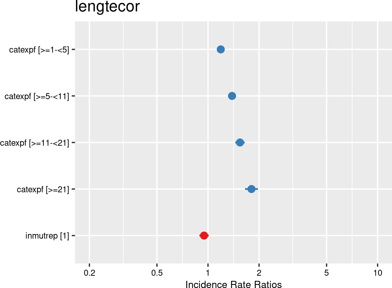

Work experience categories were introduced as fixed effects, and companies and employees as random effects. The model is based on data of all mutual Liantis ESPP and PS customers. The model is adjusted for representativeness of the company (fixed effect inmutrep) regarding to sector, size and Flemish province.
Figure 3.34 (a) and Figure 3.34 (b) demonstrate that seniority does seem to be a significant determinant for the direct wage cost of an OA for an employer.
This finding logically follows from previous models that established a significant relationship with absenteeism. Additionally, the relationship between seniority and pay level reinforces this result.
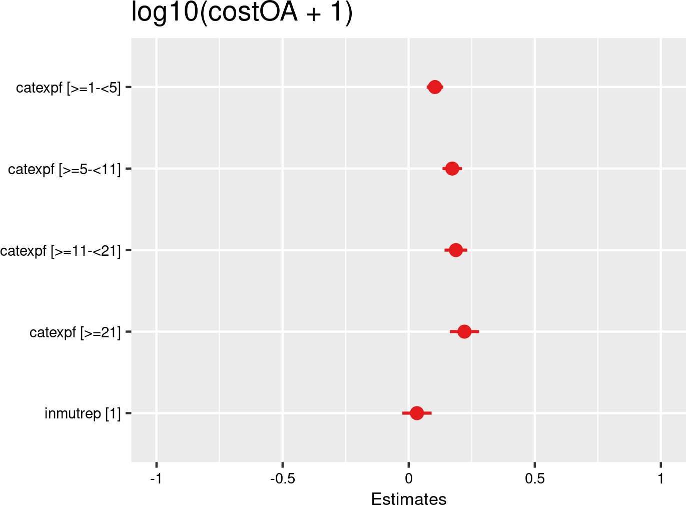

Work experience categories were introduced as fixed effects, and companies and employees as random effects. The model is based on data of all mutual Liantis ESPP and PS customers. The model is adjusted for representativeness of the company (fixed effect inmutrep) regarding to sector, size and Flemish province.
The next 4 figures (Figure 3.35 (a), Figure 3.35 (b), Figure 3.36 (a) and Figure 3.36 (b)) are displaying the results of a model assessing the relation between proportion of workers within a seniority category and the severity degree of a company, which is again a variable at the company level. In the first model ((Figure 3.35 (a) and Figure 3.35 (b)), validated number of absenteeism days from FEDRIS were used, while the second model (Figure 3.36 (a) and Figure 3.36 (b)) was based on the numbers of days off in the Liantis PS data.
From Figure 3.35 (a) and Figure 3.35 (b), a non-signicant trend that increasing fractions of people with higher seniority is associated higher severity degrees in companies can be observed.
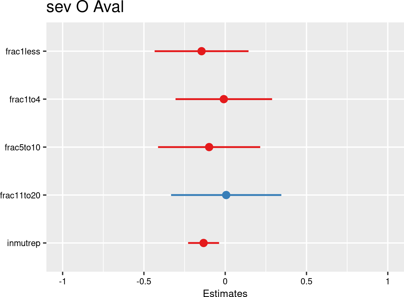

Work experience category proportions were introduced as fixed effects, and companies as random effects. The model is based on data of all mutual Liantis ESPP and PS customers. The model is adjusted for representativeness of the company (fixed effect inmutrep) regarding to sector, size and Flemish province.
From Figure 3.36 (a) and Figure 3.36 (b), the same trend, but somewhat clearer than in former model (based on FEDRIS absenteeism days), can be noticed. This is in line with the findings of models 6 and 6.1.
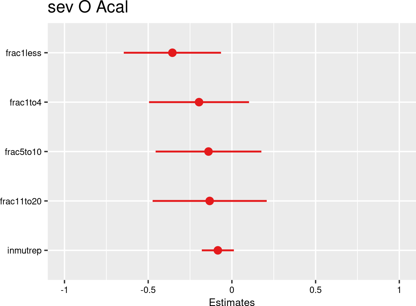

Work experience category proportions were introduced as fixed effects, and companies as random effects. The model is based on data of all mutual Liantis ESPP and PS customers. The model is adjusted for representativeness of the company (fixed effect inmutrep) regarding to sector, size and Flemish province.
3.4.1.4 Nationality (foreign workers)
3.4.1.4.1 Descriptives
International research demonstrate that foreign workers have an increased risk of (both non-fatal and fatal) occupational injures compared to the native workers (Hargreaves et al., 2019).
We used several variables as proxies to determine ‘immigrant worker’ status. First, the statistical reports from FEDRIS provide data on employee nationality in four categories: Belgium, Neighbouring Country, Other Country, and Undetermined/Unknown. Unfortunately, NSSO does not provide data on employee nationality. The Liantis PS data includes the country of birth and the INSZ (RN/BIS) number, allowing us to categorize employees into the same four categories as above. While the notifications do not provide a country of birth, they do include an INSZ (RN/BIS) number, enabling us to use them at least as a proxy for the nationality categories. Consequently, no direct match can be made between the derived category and the corresponding nationality classification.
In the next 6 tables, an overview of all (accepted) OAs (Table 3.31 and Table 3.32), the commuting OAs (Table 3.33 and Table 3.34) and the workplace OAs (Table 3.35 and Table 3.36) are given. In the first table ((Table 3.31, Table 3.33 and Table 3.35), the absolute numbers are provided stratified per nationality category, next to the total number of employees, as available in the Liantis PS database. As mentioned above, the NSSO does not provide information about nationality. In the second table (Table 3.32, Table 3.34 and Table 3.36), the relative numbers of the OAs per nationality category are provided as percentages.
From the table Table 3.32, it can be noticed that while workers from neighbours countries and other countries account for 2.5% and 7% of employees within Liantis customers, they account for about 3 and 9% of OA notifications.
all accepted occupational accidents
| nation | rszall | rszpriv | liaall | fedrisall | totalnot | totalnotmut | totalnotrepmutflan |
|---|---|---|---|---|---|---|---|
| Belgium | NA | NA | 15073793 | 1163793 | 36778 | 36778 | 16272 |
| Neighbour country | NA | NA | 454276 | 64086 | 1433 | 1433 | 455 |
| Other country | NA | NA | 1583601 | 125211 | 4359 | 4359 | 1939 |
| Undetermined/Unknown | NA | NA | 944196 | 287 | 1310 | 1310 | 408 |
| nation | percrszall | percrszpriv | percliaall | percfedrisall | perctotalnot | perctotalnotmut | perctotalnotrepmutflan |
|---|---|---|---|---|---|---|---|
| Belgium | NA | NA | 83.48 | 85.99 | 83.81 | 83.81 | 85.31 |
| Neighbour country | NA | NA | 2.52 | 4.74 | 3.27 | 3.27 | 2.39 |
| Other country | NA | NA | 8.77 | 9.25 | 9.93 | 9.93 | 10.17 |
| Undetermined/Unknown | NA | NA | 5.23 | 0.02 | 2.99 | 2.99 | 2.14 |
commuting accepted occupational accidents
| nation | rszall | rszpriv | liaall | fedrisall | totalnot | totalnotmut | totalnotrepmutflan |
|---|---|---|---|---|---|---|---|
| Belgium | NA | NA | 15073793 | 198019 | 5185 | 5185 | 2566 |
| Neighbour country | NA | NA | 454276 | 8244 | 128 | 128 | 45 |
| Other country | NA | NA | 1583601 | 19996 | 625 | 625 | 315 |
| Undetermined/Unknown | NA | NA | 944196 | 51 | 179 | 179 | 68 |
| nation | percrszall | percrszpriv | percliaall | percfedrisall | perctotalnot | perctotalnotmut | perctotalnotrepmutflan |
|---|---|---|---|---|---|---|---|
| Belgium | NA | NA | 83.48 | 87.50 | 84.76 | 84.76 | 85.70 |
| Neighbour country | NA | NA | 2.52 | 3.64 | 2.09 | 2.09 | 1.50 |
| Other country | NA | NA | 8.77 | 8.84 | 10.22 | 10.22 | 10.52 |
| Undetermined/Unknown | NA | NA | 5.23 | 0.02 | 2.93 | 2.93 | 2.27 |
workplace accepted occupational accidents
| nation | rszall | rszpriv | liaall | fedrisall | totalnot | totalnotmut | totalnotrepmutflan |
|---|---|---|---|---|---|---|---|
| Belgium | NA | NA | 15073793 | 965774 | 31593 | 31593 | 13706 |
| Neighbour country | NA | NA | 454276 | 55842 | 1305 | 1305 | 410 |
| Other country | NA | NA | 1583601 | 105215 | 3734 | 3734 | 1624 |
| Undetermined/Unknown | NA | NA | 944196 | 236 | 1131 | 1131 | 340 |
| nation | percrszall | percrszpriv | percliaall | percfedrisall | perctotalnot | perctotalnotmut | perctotalnotrepmutflan |
|---|---|---|---|---|---|---|---|
| Belgium | NA | NA | 83.48 | 85.69 | 83.66 | 83.66 | 85.24 |
| Neighbour country | NA | NA | 2.52 | 4.95 | 3.46 | 3.46 | 2.55 |
| Other country | NA | NA | 8.77 | 9.34 | 9.89 | 9.89 | 10.10 |
| Undetermined/Unknown | NA | NA | 5.23 | 0.02 | 2.99 | 2.99 | 2.11 |
3.4.1.4.2 Models
The following Table 3.37 summarizes the results of the models assessing the relationship between nationality categories and the several outcomes related to OAs. Below the table, details are provided about the data used for the analyses. The results of the nine models are then presented both graphically and in a table.
| catnation | chance to notify | chance on refusal | chance commuting | chance workplace | freq degree | chance serious | nDays TAO V/C | cost | sev degree V/C |
|---|---|---|---|---|---|---|---|---|---|
| Belgian | REF | REF | REF | REF | ns | REF | REF | REF | ns/> |
| Neighbour | > | ns | ns | > | ns | ns | >/ns | > | ns/ns |
| Other | > | ns | ns | > | ns | ns | >/ns | > | >/> |
| Undet | < | ns | < | < | rank def | ns | ns/ns | < | rank def |
| occur | accept | occur | occur | occur | severe | severe | severe | severe | |
| empl | empl | empl | empl | comp | empl | empl | empl | comp | |
| c/w all | c/w ref | c acc | w acc | w acc | w acc | w acc | w acc | w acc |
- occur: data include all workers, chance for occurrence is calculated for the outcome
- accept: data include only workers with a notification of OA
- severe: data include only workers with an accepted OA
- c/w all: commuting and workplace accidents, including refused and accidents without decisions
- c/w ref: accepted or refused commuting and workplace accidents
- c acc: accepted commuting accidents
- w acc: accepted workplace accidents
- empl: the outcome is situated at the individual level
- comp: the outcome is situated at the company level
- nDaysTAO: number of days absenteeism related to the OA
- V/C: Validated number of days (available from FEDRIS) / Calculated number of days (based on the Liantis PS data)
Nationality (foreign workers) and occupational accidents
- Workers from other countries seem to have a higher likelihood of experiencing workplace accidents in comparison with the nationals.
- There was no relation between nationality and the chance for an occupational accident to be categorized as serious.
- For the companies, we did not find a relation between proportion of foreign workers and the frequency degree. There was a positive relation between a higher proportion of workers from countries apart from neighbours and a higher severity degree.
- The (validated but not calculated) number of days off related to an occupational accident is significantly higher in workers from a neighbour or other country and also reflected in the direct wage cost.
According to Figure 3.37 (a) and Figure 3.37 (b), workers from another country have a 20% to 22% higher chance to report an OA (both commuting and workplace accidents) than the reference category of Belgian workers (after accounting for significant differences in representativeness of the company). This is in line with literature that highlights that migrants are more often involved in OAs than natives (Ahonen, 2006; Ahonen & Benavides, 2016; Guerreschi et al., 2024; Hargreaves et al., 2019; Salminen, 2011).
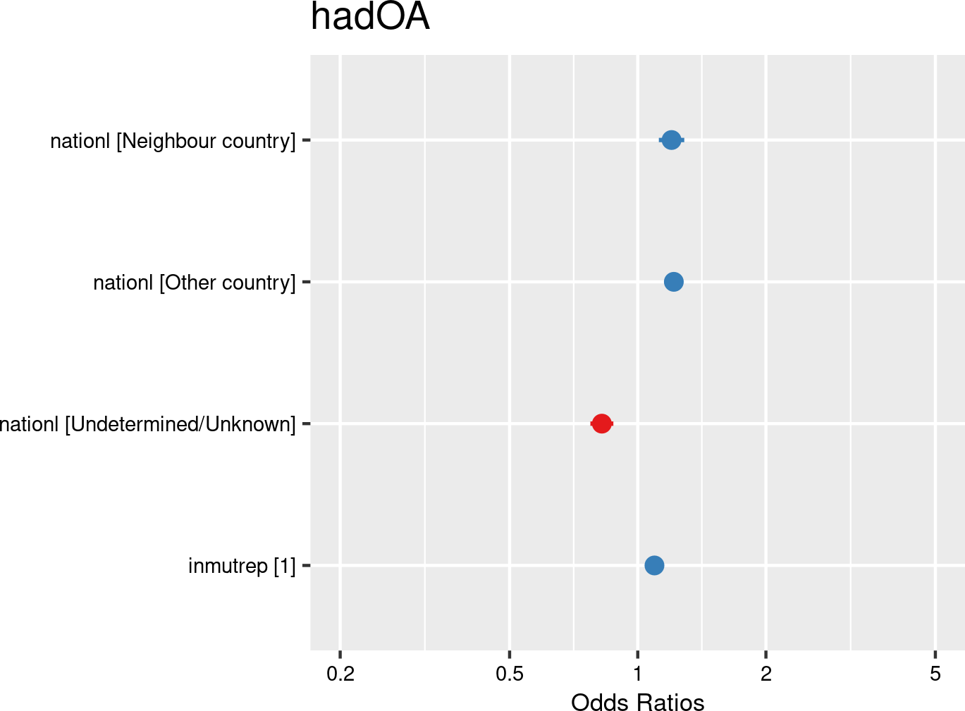

Nationality categories were introduced as fixed effects, and companies and employees as random effects. The model is based on data from employees with and without OAs from all mutual Liantis ESPP and PS customers. The model is adjusted for representativeness of the company (fixed effect inmutrep) regarding to sector, size and Flemish province.
From Figure 3.38 (a) and Figure 3.38 (b) it can be concluded that nationality does not seem to be an important determinant for acceptance or refusal of an OA by an insurer. This is in line with expectations: we do not expect that based on nationality an OA would be accepted or refused.
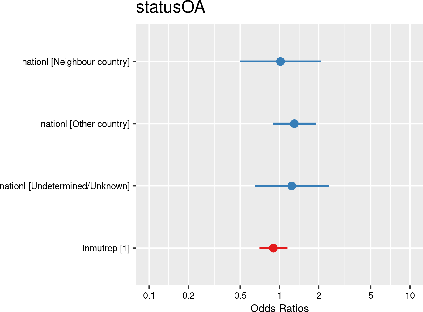

Nationality categories were introduced as fixed effects, and companies and employees as random effects. The model is based on data from employees notifying OAs from all mutual Liantis ESPP and PS customers. The model is adjusted for representativeness of the company (fixed effect inmutrep) regarding to sector, size and Flemish province.
Figure 3.39 (a) and Figure 3.39 (b) shows that workers from other countries do not experience an higher chance for an accepted commuting accident in comparison with nationals. The literature review did not provide a clear conclusion regarding this relationship, nor do our results.
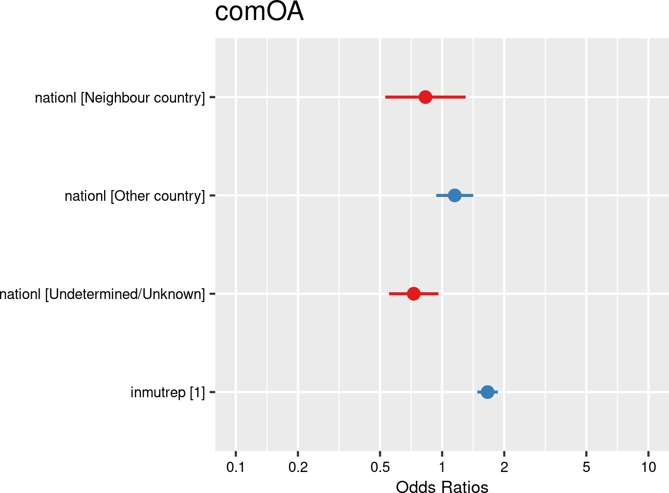

Nationality categories were introduced as fixed effects, and companies and employees as random effects. The model is based on data from employees with and without OAs from all mutual Liantis ESPP and PS customers. The model is adjusted for representativeness of the company (fixed effect inmutrep) regarding to sector, size and Flemish province.
According Figure 3.40 (a) and Figure 3.40 (b), workers from countries show a 20% to 24% higher chance on an accepted workplace OA than the nationals (after accounting for significant differences in representativeness of the company). As previously mentioned, this aligns with the findings from the literature on this topic (Ahonen, 2006; Ahonen & Benavides, 2016; Guerreschi et al., 2024; Hargreaves et al., 2019; Salminen, 2011).


Nationality categories were introduced as fixed effects, and companies and employees as random effects. The model is based on data from employees with and without OAs from all mutual Liantis ESPP and PS customers. The model is adjusted for representativeness of the company (fixed effect inmutrep) regarding to sector, size and Flemish province.
Figure 3.41 (a) and Figure 3.41 (b) present a model estimating the frequency degree of OAs at the company level, in contrast to previous models that focused on individual employee accident probabilities. These figures show that the proportion of workers who are nationals, from neighbouring countries, or from other countries is not related to the company’s accident frequency. While one might hypothesize that companies employing many immigrant workers or those with a mother tongue other than Dutch or French might experience more accidents, this analysis did not reveal such a pattern.
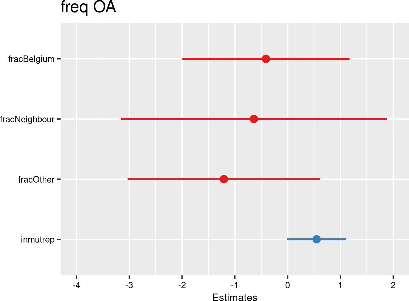

Nationality category proportions were introduced as fixed effects, and companies as random effects. The model is based on data of all mutual Liantis ESPP and PS customers. The model is adjusted for representativeness of the company (fixed effect inmutrep) regarding to sector, size and Flemish province.
According to Figure 3.42 (a) and Figure 3.42 (b), nationality does not appear to be a significant factor in classifying an workplace OA as serious. This contrasts somewhat with literature findings that suggest a higher risk of serious and fatal OAs among migrant workers (Ahonen, 2006; Ahonen & Benavides, 2016; Guerreschi et al., 2024; Hargreaves et al., 2019). However, it’s important to note that our analysis defines a serious accident according to Belgian law, which may differ considerably from definitions used in the literature. Additionally, our analysis focused on workers with accepted OAs (modelling the risk that an OA is classified as serious), whereas the literature often models the likelihood of experiencing a serious OA.
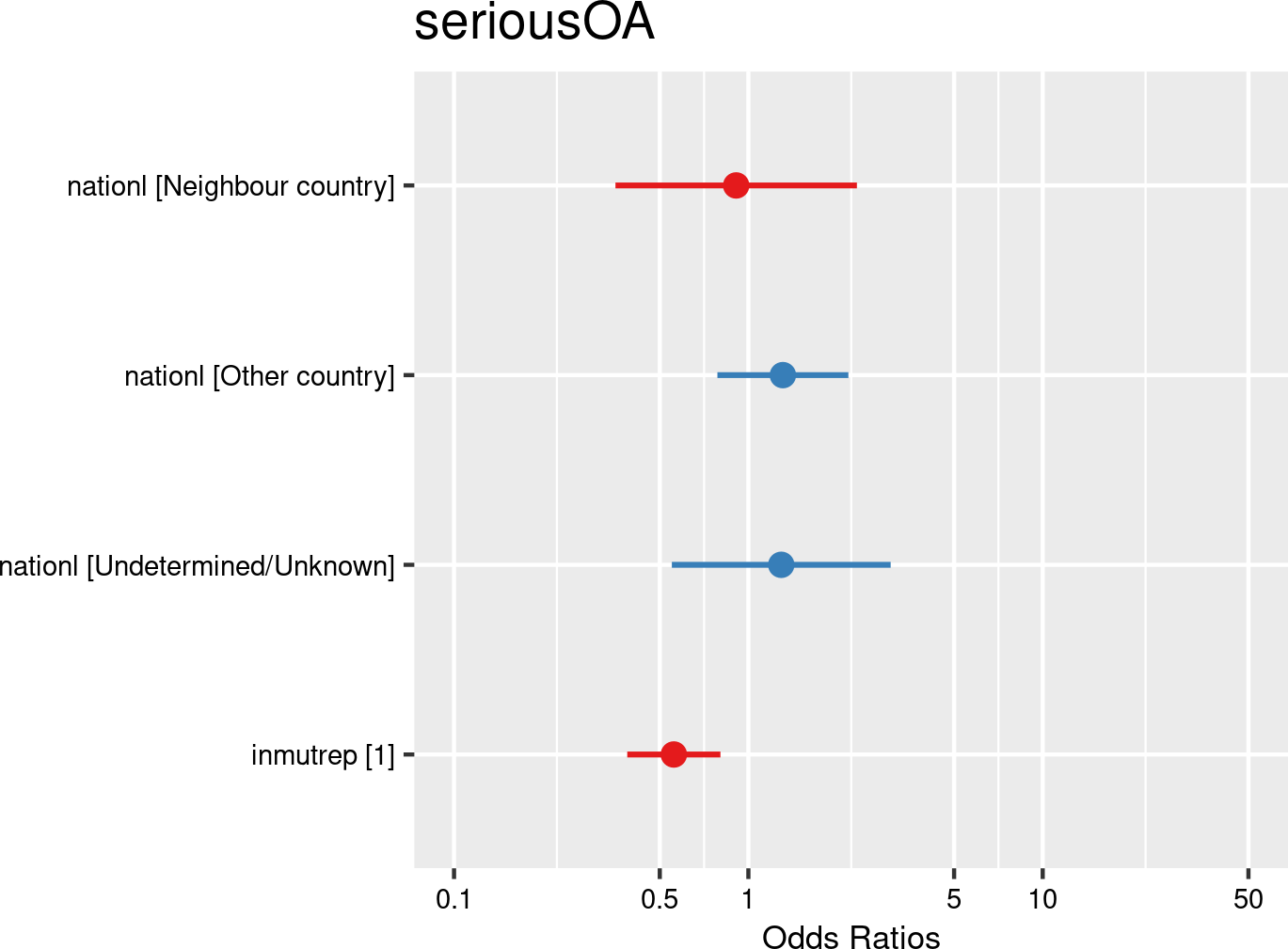

Nationality categories were introduced as fixed effects, and companies and employees as random effects. The model is based on data of all mutual Liantis ESPP and PS customers. The model is adjusted for representativeness of the company (fixed effect inmutrep) regarding to sector, size and Flemish province.
Figure 3.43 (a) and Figure 3.43 (b) are the results of a model assessing the relation between nationality and the number of absenteeism days. These first 2 figures are based on the absenteeism data provided by FEDRIS (while Figure 3.44 (a) and Figure 3.44 (b) present the same model based on the Liantis PS data). These figures show that nationality is an important factor in determining the validated number of absenteeism days related to the OA. A worker from a neighbourhood country has on average a 20% increase in absenteeism days in comparison with the Belgian worker, while workers from other than neighbour countries show 12% more absenteeism days.
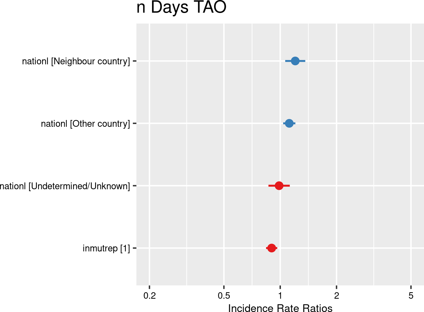

Nationality categories were introduced as fixed effects, and companies and employees as random effects. The model is based on data of all mutual Liantis ESPP and PS customers. The model is adjusted for representativeness of the company (fixed effect inmutrep) regarding to sector, size and Flemish province.
The next two figures (Figure 3.44 (a) and Figure 3.44 (b)) showing the calculated number of absenteeism days (from the Liantis PS data) related to the OA however did not confirm the previous significant findings between nationality and validated absenteeism days (from FEDRIS). These inconsistent findings may be due to differences in the study populations between the Liantis PS data and the FEDRIS absenteeism data (e.g. the Liantis PS dataset being considerably smaller).
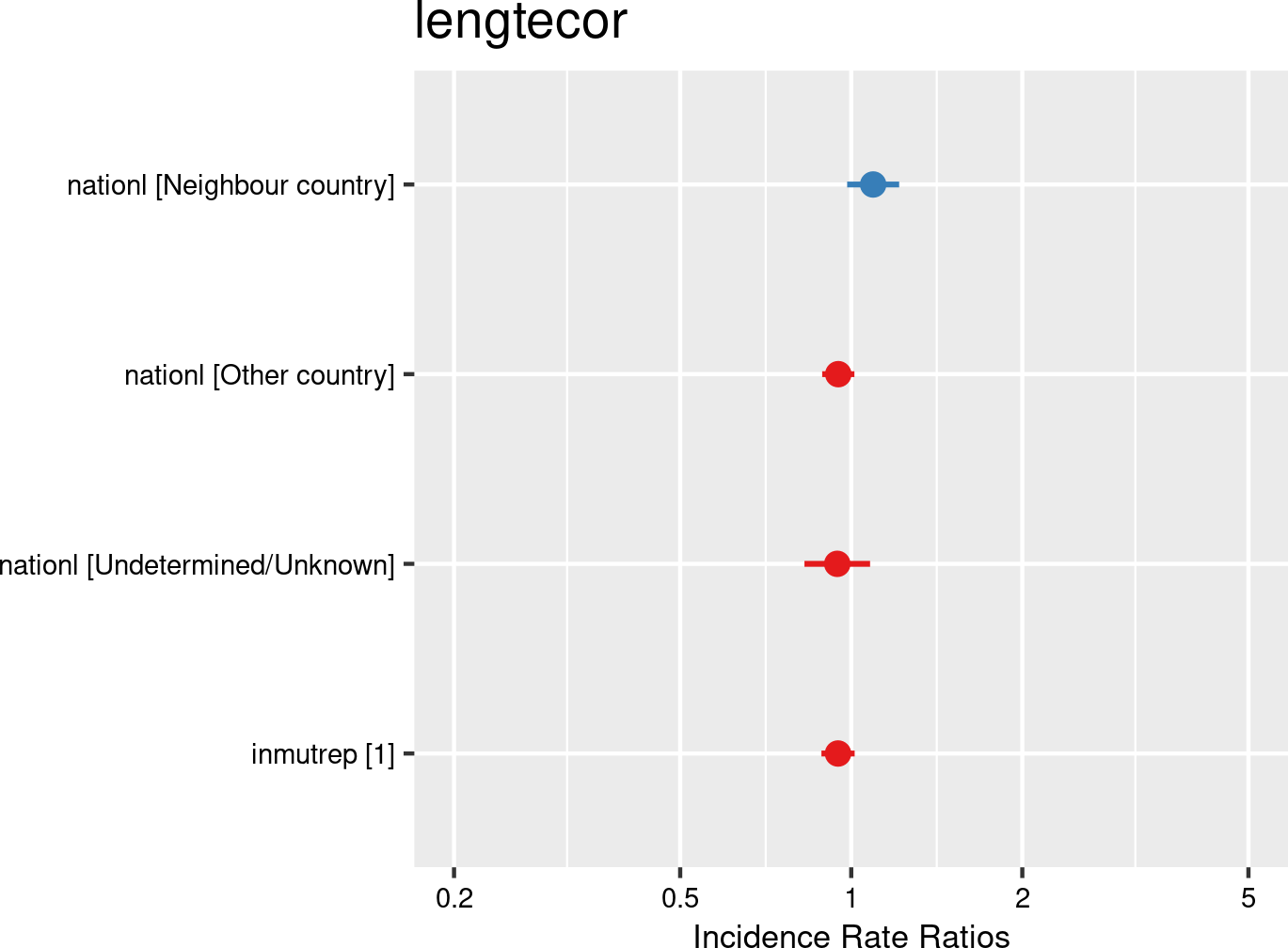

Nationality categories were introduced as fixed effects, and companies and employees as random effects. The model is based on data of all mutual Liantis ESPP and PS customers. The model is adjusted for representativeness of the company (fixed effect inmutrep) regarding to sector, size and Flemish province.
According to Figure 3.45 (a) and Figure 3.45 (b), workers from other countries incur significantly higher direct wage costs (in comparison with nationals) for employers due to OAs.
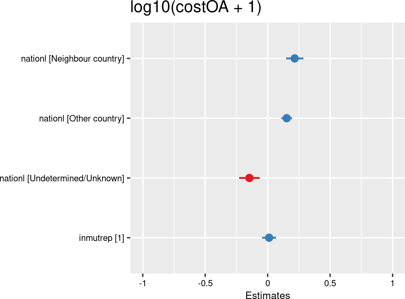

Nationality categories were introduced as fixed effects, and companies and employees as random effects. The model is based on data of all mutual Liantis ESPP and PS customers. The model is adjusted for representativeness of the company (fixed effect inmutrep) regarding to sector, size and Flemish province.
The next 4 figures (Figure 3.46 (a), Figure 3.46 (b), Figure 3.47 (a) and Figure 3.47 (b)) are displaying the results of a model assessing the relation between the proportion of workers within a nationality category and the severity degree of a company, which is again a variable at the company level. In the first model ((Figure 3.46 (a) and Figure 3.46 (b)), validated number of absenteeism days from FEDRIS were used for the calculation of the severity degree, while the second model (Figure 3.47 (a) and Figure 3.47 (b)) was based on the numbers of days off in the Liantis PS data.
From Figure 3.46 (a) and Figure 3.46 (b), it can be inferred that a higher proportion of workers from countries other than neighbouring ones is associated with a higher severity degree in companies.
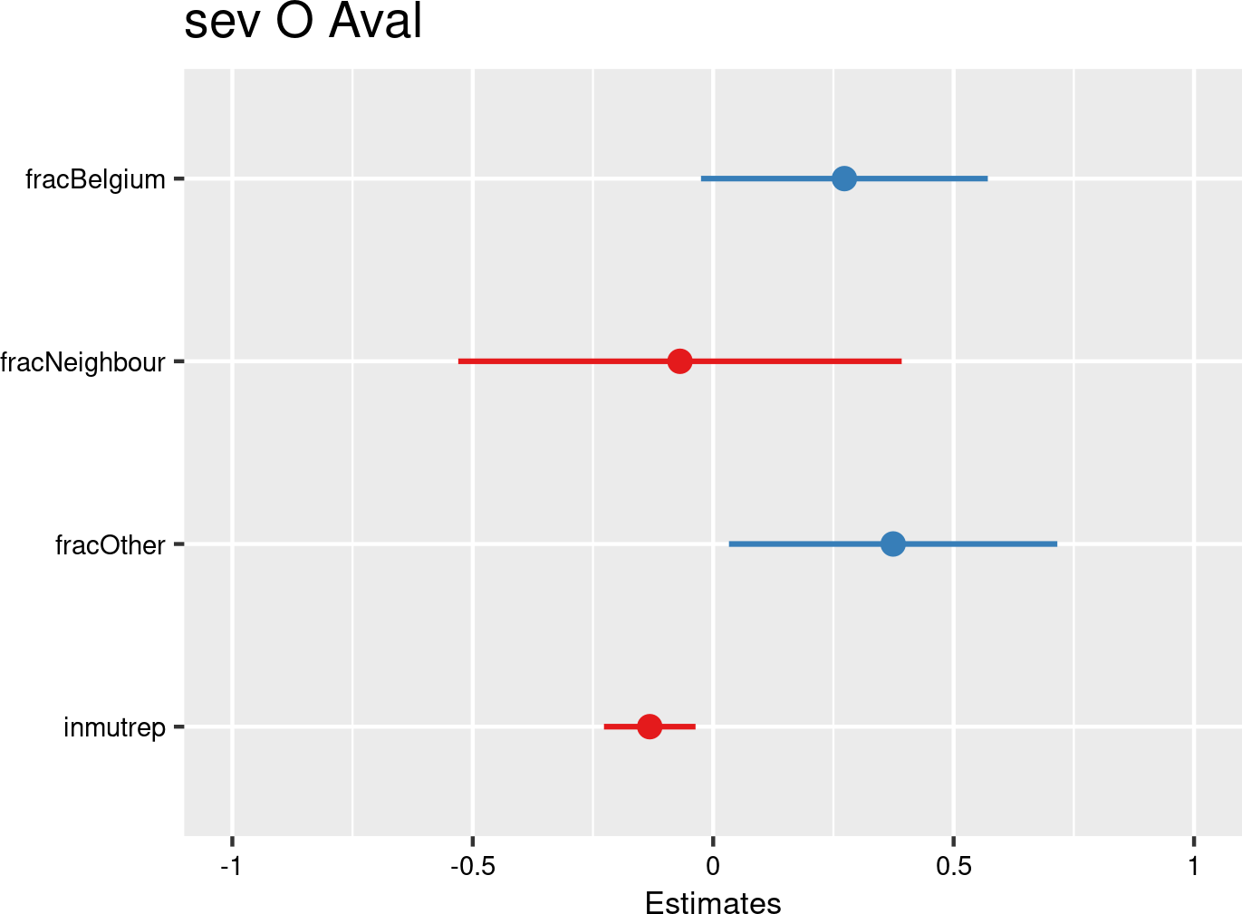

Nationality category proportions were introduced as fixed effects, and companies as random effects. The model is based on data of all mutual Liantis ESPP and PS customers. The model is adjusted for representativeness of the company (fixed effect inmutrep) regarding to sector, size and Flemish province.
The analysis based on the number of absenteeism days in the Liantis PS data (Figure 3.47 (a) and Figure 3.47 (b)) also shows a significant positive relationship between the proportion of workers from non-neighbouring countries and the severity degree of a company. Additionally, a positive relationship was found for the proportion of Belgian workers. However, these findings may be influenced by differences in the sample populations.
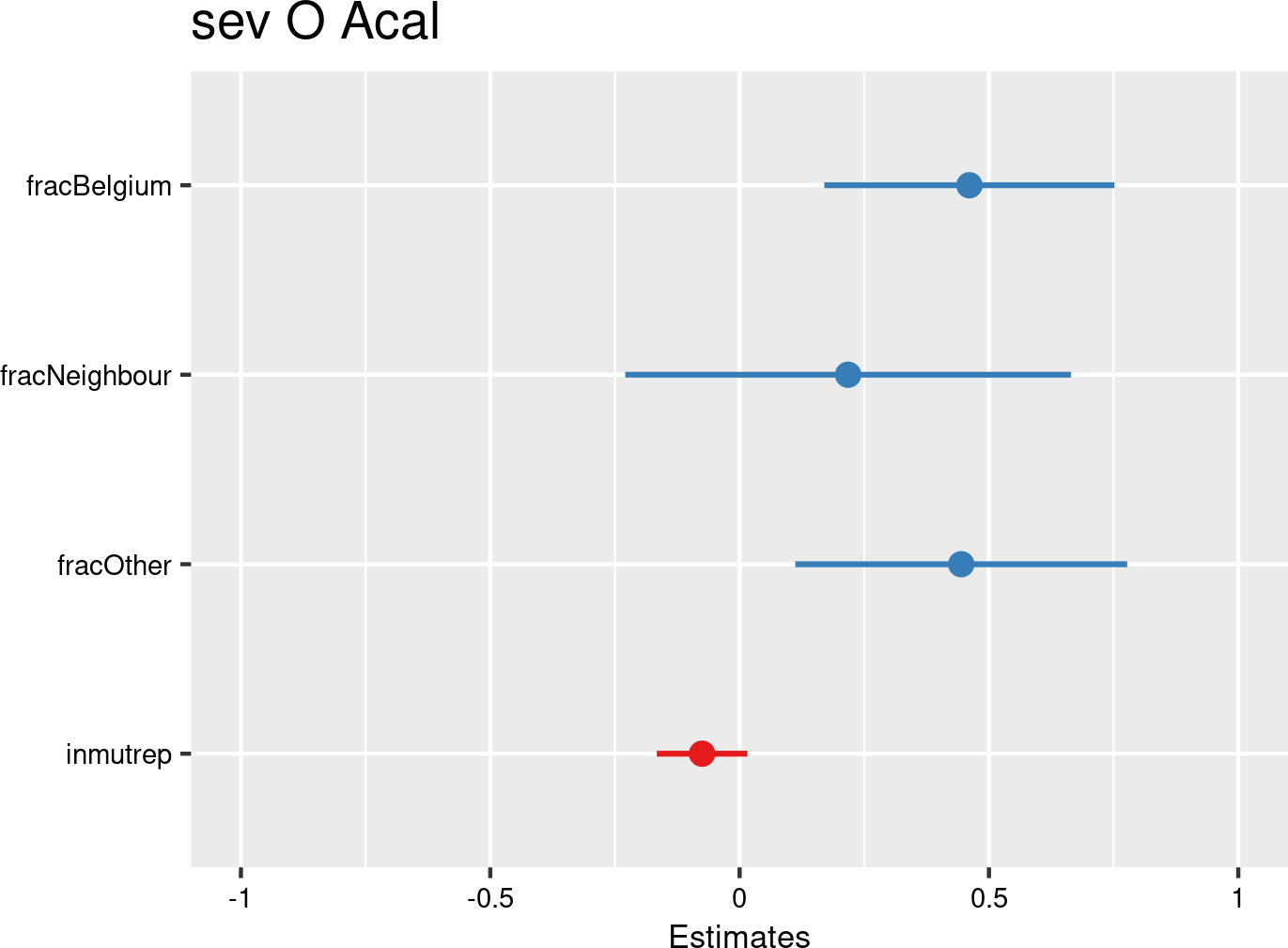

Nationality category proportions were introduced as fixed effects, and companies as random effects. The model is based on data of all mutual Liantis ESPP and PS customers. The model is adjusted for representativeness of the company (fixed effect inmutrep) regarding to sector, size and Flemish province.
3.4.1.5 Salary level
3.4.1.5.1 Descriptives
We used the day wage as a proxy for salary. The NSSO provides statistics on the day wage of employees in 12 categories, which we regrouped into seven categories (<€50, €50-99, €100-124, €125-149, €150-199, €200-249, \(\geq\) €250). The Liantis PS data includes the hourly wage (derived through the division of the brute wage and the effectively worked hours), which allows us to derive the day wage of employees by multiplying the hourly wage by 7.6 (equivalent to the day wage of a full-time worker). However, the notifications do not provide any salary or wage information of the employee. Since this information is absent in the notifications passed through to Liantis, the comparison with the derived wage of an employee experiencing an OA cannot be made.
A reference category of day wages below €50 should be interpreted with caution
Employees with a day wage of <€50 are likely to be part-time workers, temporary workers, or workers with very low working hours. Therefore, this category may not accurately represent low-wage full-time employees. Caution is advised when interpreting results related to this wage category. It was challenging to join and compare globalised NSSO data with detailed Liantis data. The risk exists that we are trying to compare very different things. The authors do believe that the relative differences between the categories are informative, but caution is needed when interpreting and certain data quality issues will be need to considered. For more details, see Section 3.6 on limitations and strenghts.
In the next 6 tables, an overview of all (accepted) OAs (Table 3.38 and Table 3.39), the commuting OAs (Table 3.40 and Table 3.41) and the workplace OAs (Table 3.42 and Table 3.43) are given. In the first table ((Table 3.38, Table 3.40 and Table 3.42), the absolute numbers are provided stratified per wage category, next to the total number of employees, as available in the Liantis PS database. In the second table (Table 3.39, Table 3.41 and Table 3.43), the relative numbers of the OAs per wage category are provided as percentages.
From the table Table 3.39, it can be noticed that while workers in the wage category <50 euro, and \(\geq\) 205 euro, account for respectively 19% and 9% of the employees within Liantis customers, they account for 4.4% and 4.6% of the employees within the notifications. The opposite pattern can be noticed for the workers in the wage category 100-124 euro and 150-199 euro: they account for respectively 20 and 12% of the employees within Liantis customers, while they account for 32.9 and 18.3% of the workers within the notifications.
all accepted occupational accidents
| catwage | rszall | rszpriv | liaall | fedrisall | totalnot | totalnotmut | totalnotrepmutflan |
|---|---|---|---|---|---|---|---|
| < 50 | 1244217.79 | 1134679.33 | 3404294 | NA | 1910 | 1910 | 657 |
| 50 - 99 | 19876144.04 | 17520360.55 | 4275137 | NA | 11059 | 11059 | 4455 |
| 100 - 124 | 28050533.65 | 22741692.40 | 3625308 | NA | 14445 | 14445 | 5598 |
| 125 - 149 | 24670336.11 | 18466319.81 | 2227516 | NA | 8015 | 8015 | 3427 |
| 150 - 199 | 29640188.47 | 19089420.83 | 2040008 | NA | 4775 | 4775 | 2733 |
| 200 - 249 | 12467321.44 | 8014278.56 | 796203 | NA | 1653 | 1653 | 1110 |
| >= 250 | 10098764.90 | 7273469.82 | 1687400 | NA | 2023 | 2023 | 1094 |
| Unknown | 38353.87 | 37133.66 | 0 | NA | 151339 | 17355 | 6956 |
| catwage | percrszall | percrszpriv | percliaall | percfedrisall | perctotalnot | perctotalnotmut | perctotalnotrepmutflan |
|---|---|---|---|---|---|---|---|
| < 50 | 1.0 | 1.2 | 18.9 | NA | 4.4 | 4.4 | 3.4 |
| 50 - 99 | 15.8 | 18.6 | 23.7 | NA | 25.2 | 25.2 | 23.4 |
| 100 - 124 | 22.3 | 24.1 | 20.1 | NA | 32.9 | 32.9 | 29.3 |
| 125 - 149 | 19.6 | 19.6 | 12.3 | NA | 18.3 | 18.3 | 18.0 |
| 150 - 199 | 23.5 | 20.3 | 11.3 | NA | 10.9 | 10.9 | 14.3 |
| 200 - 249 | 9.9 | 8.5 | 4.4 | NA | 3.8 | 3.8 | 5.8 |
| >= 250 | 8.0 | 7.7 | 9.3 | NA | 4.6 | 4.6 | 5.7 |
| Unknown | NA | NA | NA | NA | NA | NA | NA |
commuting accepted occupational accidents
| catwage | rszall | rszpriv | liaall | fedrisall | totalnot | totalnotmut | totalnotrepmutflan |
|---|---|---|---|---|---|---|---|
| < 50 | 1244217.79 | 1134679.33 | 3404294 | NA | 277 | 277 | 113 |
| 50 - 99 | 19876144.04 | 17520360.55 | 4275137 | NA | 1850 | 1850 | 802 |
| 100 - 124 | 28050533.65 | 22741692.40 | 3625308 | NA | 1563 | 1563 | 717 |
| 125 - 149 | 24670336.11 | 18466319.81 | 2227516 | NA | 889 | 889 | 454 |
| 150 - 199 | 29640188.47 | 19089420.83 | 2040008 | NA | 858 | 858 | 483 |
| 200 - 249 | 12467321.44 | 8014278.56 | 796203 | NA | 347 | 347 | 233 |
| >= 250 | 10098764.90 | 7273469.82 | 1687400 | NA | 333 | 333 | 192 |
| Unknown | 38353.87 | 37133.66 | 0 | NA | 22270 | 2482 | 1118 |
| catwage | percrszall | percrszpriv | percliaall | percfedrisall | perctotalnot | perctotalnotmut | perctotalnotrepmutflan |
|---|---|---|---|---|---|---|---|
| < 50 | 1.0 | 1.2 | 18.9 | NA | 4.5 | 4.5 | 3.8 |
| 50 - 99 | 15.8 | 18.6 | 23.7 | NA | 30.2 | 30.2 | 26.8 |
| 100 - 124 | 22.3 | 24.1 | 20.1 | NA | 25.6 | 25.6 | 23.9 |
| 125 - 149 | 19.6 | 19.6 | 12.3 | NA | 14.5 | 14.5 | 15.2 |
| 150 - 199 | 23.5 | 20.3 | 11.3 | NA | 14.0 | 14.0 | 16.1 |
| 200 - 249 | 9.9 | 8.5 | 4.4 | NA | 5.7 | 5.7 | 7.8 |
| >= 250 | 8.0 | 7.7 | 9.3 | NA | 5.4 | 5.4 | 6.4 |
| Unknown | NA | NA | NA | NA | NA | NA | NA |
workplace accepted occupational accidents
| catwage | rszall | rszpriv | liaall | fedrisall | totalnot | totalnotmut | totalnotrepmutflan |
|---|---|---|---|---|---|---|---|
| < 50 | 1244217.79 | 1134679.33 | 3404294 | NA | 1633 | 1633 | 544 |
| 50 - 99 | 19876144.04 | 17520360.55 | 4275137 | NA | 9209 | 9209 | 3653 |
| 100 - 124 | 28050533.65 | 22741692.40 | 3625308 | NA | 12882 | 12882 | 4881 |
| 125 - 149 | 24670336.11 | 18466319.81 | 2227516 | NA | 7126 | 7126 | 2973 |
| 150 - 199 | 29640188.47 | 19089420.83 | 2040008 | NA | 3917 | 3917 | 2250 |
| 200 - 249 | 12467321.44 | 8014278.56 | 796203 | NA | 1306 | 1306 | 877 |
| >= 250 | 10098764.90 | 7273469.82 | 1687400 | NA | 1690 | 1690 | 902 |
| Unknown | 38353.87 | 37133.66 | 0 | NA | 129069 | 14873 | 5838 |
| catwage | percrszall | percrszpriv | percliaall | percfedrisall | perctotalnot | perctotalnotmut | perctotalnotrepmutflan |
|---|---|---|---|---|---|---|---|
| < 50 | 1.0 | 1.2 | 18.9 | NA | 4.3 | 4.3 | 3.4 |
| 50 - 99 | 15.8 | 18.6 | 23.7 | NA | 24.4 | 24.4 | 22.7 |
| 100 - 124 | 22.3 | 24.1 | 20.1 | NA | 34.1 | 34.1 | 30.4 |
| 125 - 149 | 19.6 | 19.6 | 12.3 | NA | 18.9 | 18.9 | 18.5 |
| 150 - 199 | 23.5 | 20.3 | 11.3 | NA | 10.4 | 10.4 | 14.0 |
| 200 - 249 | 9.9 | 8.5 | 4.4 | NA | 3.5 | 3.5 | 5.5 |
| >= 250 | 8.0 | 7.7 | 9.3 | NA | 4.5 | 4.5 | 5.6 |
| Unknown | NA | NA | NA | NA | NA | NA | NA |
3.4.1.5.2 Models
The following Table 3.44 table summarizes the results of the models assessing the relationship between wage categories and the several outcomes related to OAs. Below the table, details are provided about the data used for the analyses. The results of the nine models are then presented both graphically and in a table.
| catwage | chance to notify | chance on refusal | chance commuting | chance workplace | freq degree | chance serious | nDays TAO V/C | cost | sev degree V/C |
|---|---|---|---|---|---|---|---|---|---|
| <50 | REF | REF | REF | REF | ns | REF | REF | REF | >/> |
| 50-99 | > | ns | > | > | > | ns | >/ns | > | ns/> |
| 100-124 | > | ns | > | > | > | ns | >/ns | > | >/> |
| 125-149 | > | ns | > | > | > | ns | ns/ns | > | >/> |
| 150-199 | > | ns | > | > | > | ns | ns/ns | > | ns/ns |
| 200-249 | > | ns | > | > | ns | ns | ns/> | > | ns/ns |
| >=250 | > | ns | > | > | rank def | ns | </ns | > | rank def |
| occur | accept | occur | occur | occur | severe | severe | severe | severe | |
| empl | empl | empl | empl | comp | empl | empl | empl | comp | |
| c/w all | c/w ref | c acc | w acc | w acc | w acc | w acc | w acc | w acc |
- occur: data include all workers, chance for occurrence is calculated for the outcome
- accept: data include only workers with a notification of OA
- severe: data include only workers with an accepted OA
- c/w all: commuting and workplace accidents, including refused and accidents without decisions
- c/w ref: accepted or refused commuting and workplace accidents
- c acc: accepted commuting accidents
- w acc: accepted workplace accidents
- empl: the outcome is situated at the individual level
- comp: the outcome is situated at the company level
- nDaysTAO: number of days absenteeism related to the OA
- V/C: Validated number of days (available from FEDRIS) / Calculated number of days (based on the Liantis PS data)
Salary and occupational accidents
- Workers earning between €100-124 per day have the highest probability of experiencing a commuting or workplace accident. For higher wage categories, the odds decrease as the wage category increases.
- A higher proportion of workers earning between €100-124 and €125-149 significantly increases the frequency degree of occupational accidents within a company.
- Wage category does not significantly determine whether an occupational accident is classified as serious.
- Wage category is a significant factor in determining the number of absenteeism days due to occupational accidents: the number of days off is significantly higher for lower wage categories.
- A higher proportion of workers in the lowest wage categories increases the severity degree within a company.
Figure 3.48 (a) and Figure 3.48 (b) illustrate that all wage categories have a higher likelihood of reporting an OA (both commuting and workplace accidents) compared to the lowest category (<€50), even after accounting for significant differences in company representativeness. Workers earning between €100-124/day have the highest probability of reporting an OA, with odds more than seven times higher than those in the lowest wage group.
In literature, inconsistent results are found regarding the relationship between wages and the incidence of OAs. Two opposing theories are proposed: some authors suggest that higher wage groups experience a higher incidence of OAs, viewing wages as compensation for the risky nature of their jobs (Lalive, Rafael and Ruf, Oliver and Zweimuller, Josef, 2006). Conversely, other findings indicate that workers with higher wages have a lower incidence of OAs, reflecting their preference for less risky jobs (Cabrera-Flores, 2023). Both theories may be relevant to our results.
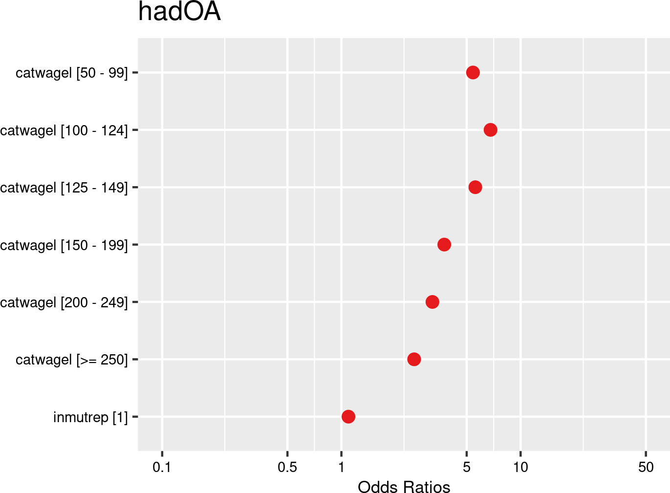

Wage categories were introduced as fixed effects, and companies and employees as random effects. The model is based on data from employees with and without OAs from all mutual Liantis ESPP and PS customers. The model is adjusted for representativeness of the company (fixed effect inmutrep) regarding to sector, size and Flemish province.
Figure 3.49 (a) and Figure 3.49 (b) show that wage category does not significantly determine whether an insurer accepts or rejects an OA claim. This is in line with expectations.
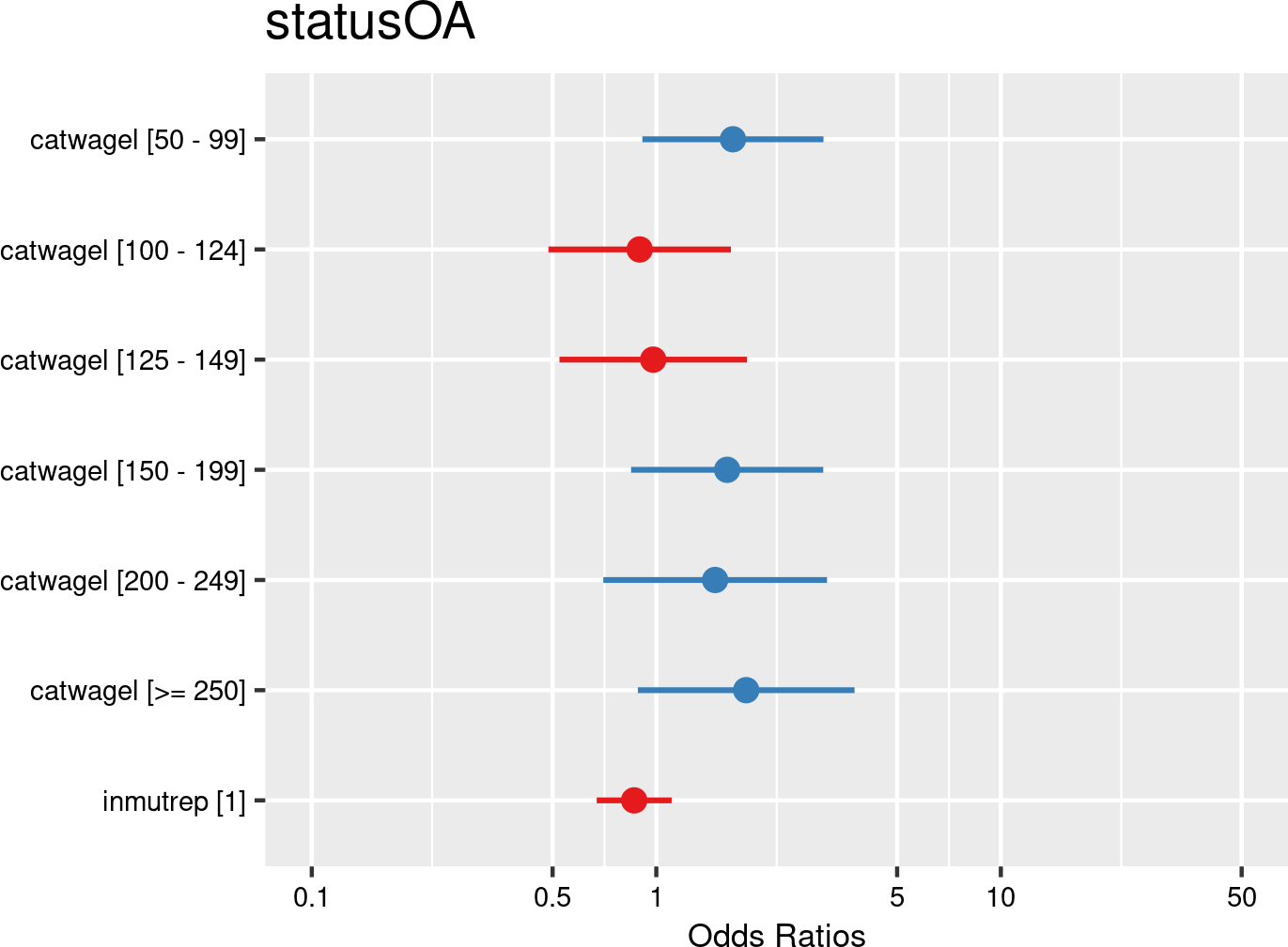

Wage categories were introduced as fixed effects, and companies and employees as random effects. The model is based on data from employees notifying OAs from all mutual Liantis ESPP and PS customers. The model is adjusted for representativeness of the company (fixed effect inmutrep) regarding to sector, size and Flemish province.
Figure 3.50 (a) and Figure 3.50 (b) show that all wage categories have a higher likelihood of an accepted commuting accident compared to the lowest wage category (<€50). However, workers earning between €100-124/day have the highest probability of experiencing a commuting accident, with odds nearly 7 times higher than those in the lowest wage group. For higher wage categories, the trend shows that the odds decrease as the wage category increases. We found no studies examining this specific relationship between wage and the likelihood of commuting occupational risk.
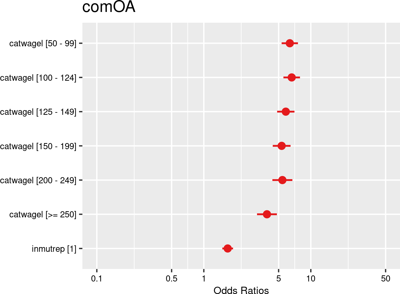

Wage categories were introduced as fixed effects, and companies and employees as random effects. The model is based on data from employees with and without OAs from all mutual Liantis ESPP and PS customers. The model is adjusted for representativeness of the company (fixed effect inmutrep) regarding to sector, size and Flemish province.
Figure 3.51 (a) and Figure 3.51 (b) show the estimates for the relation between wage categories and an accepted workplace OA. The relation is comparable of that noticed in the figures for reporting an OA. In summary, all wage categories have a higher likelihood of an accepted workplace OA, with the highest odds for the category between €100-124/day, compared to the lowest category (<€50). For higher wage categories, the trend shows that the odds decrease as the wage category increases.
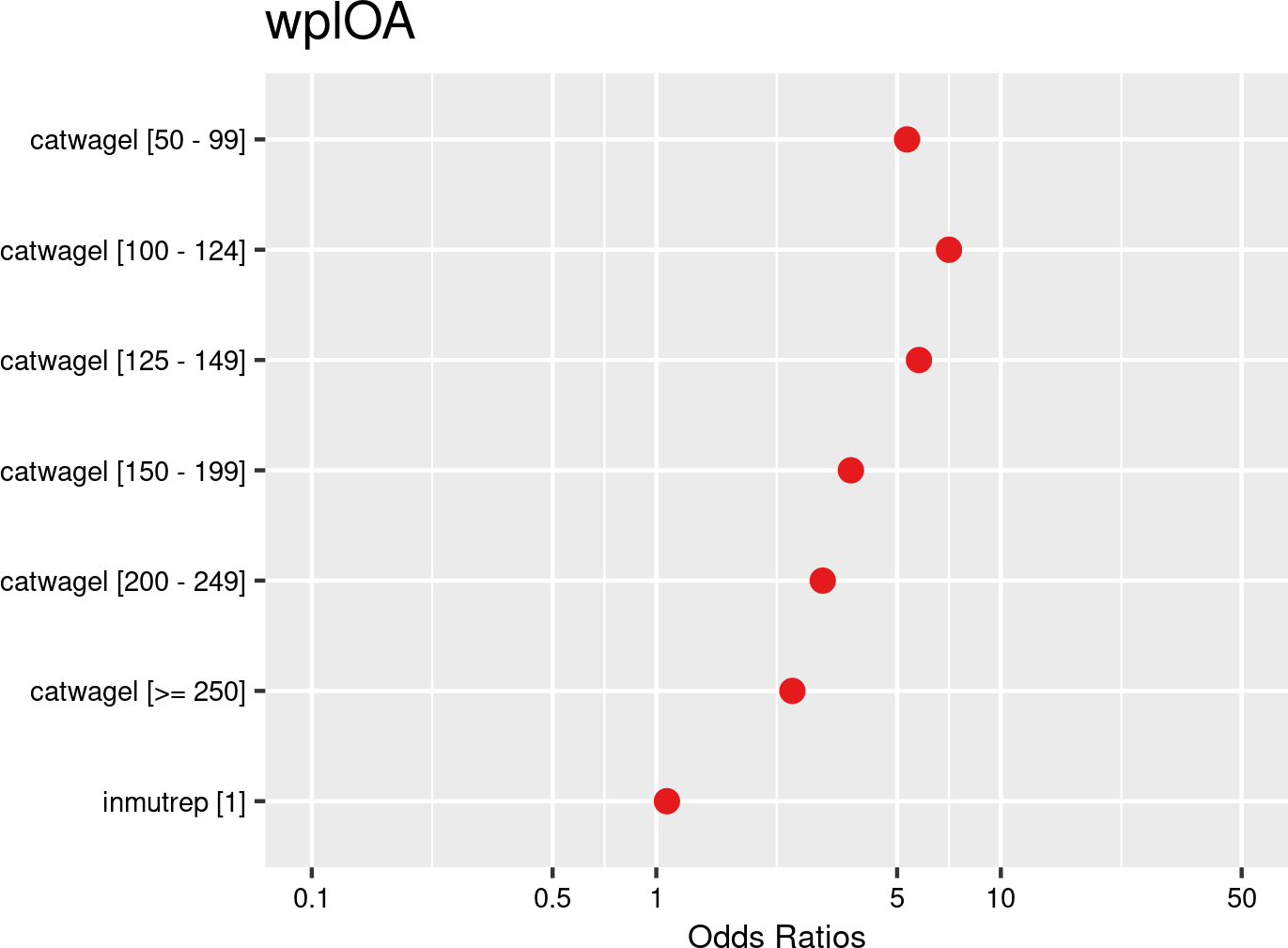

Wage categories were introduced as fixed effects, and companies and employees as random effects. The model is based on data from employees with and without OAs from all mutual Liantis ESPP and PS customers. The model is adjusted for representativeness of the company (fixed effect inmutrep) regarding to sector, size and Flemish province.
Figure 3.52 (a) and Figure 3.52 (b) present a model estimating the frequency degree of OAs at the company level, in contrast to previous models that focused on individual employee accident probabilities. These figures indicate that a higher proportion of workers earning between €100-124 and €125-149 significantly increases the frequency degree of OAs within a company.
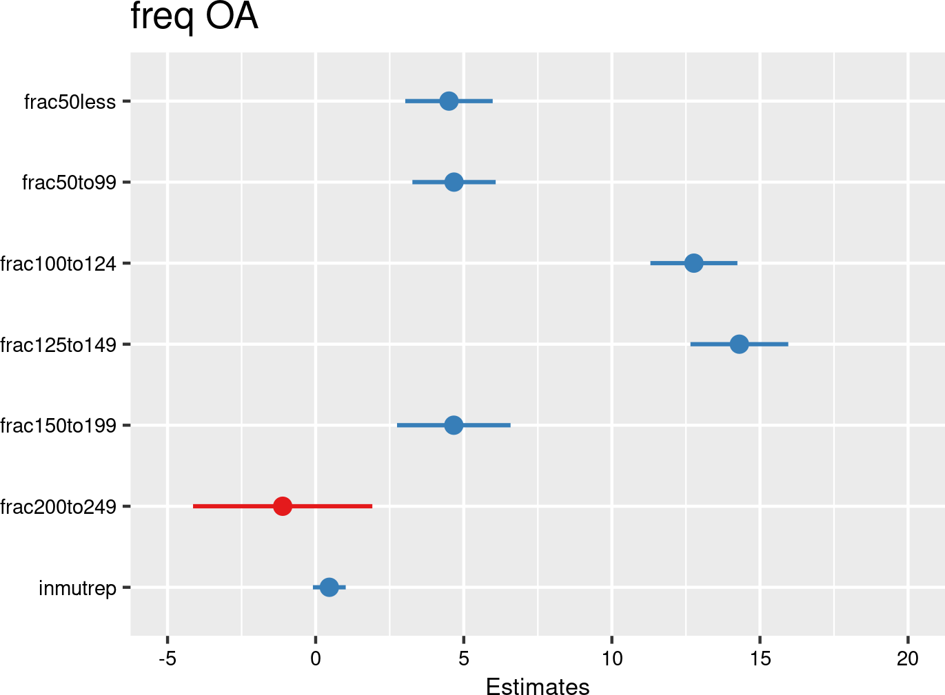

Figure 3.53 (a) and Figure 3.53 (b) present a model estimating the chance for an accepted OA being serious (according to the definition of the Belgian law). These figures indicate that wage category does not significantly determine whether a workplace OA is classified as serious. This contrasts with the wage premium theory, which suggests that workers in riskier jobs are offered higher wages. According to this theory, these higher-paid workers tend to experience more serious or fatal accidents, but fewer non-serious ones (Lalive, Rafael and Ruf, Oliver and Zweimuller, Josef, 2006). However, it’s important to note that the definition of a serious OA under Belgian law may differ from those used in literature.
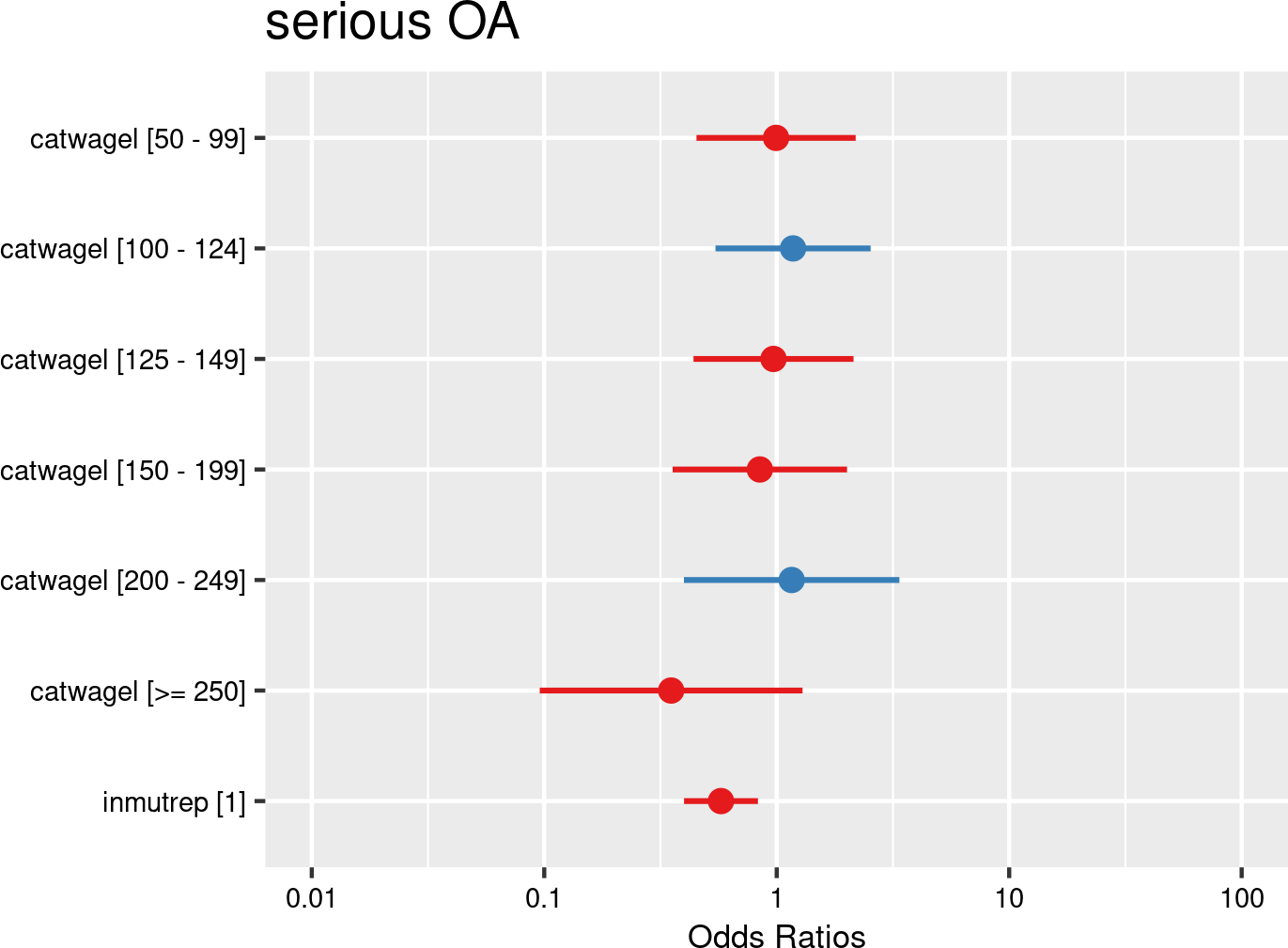

Wage categories were introduced as fixed effects, and companies and employees as random effects. The model is based on data of all mutual Liantis ESPP and PS customers. The model is adjusted for representativeness of the company (fixed effect inmutrep) regarding to sector, size and Flemish province.
Figure 3.54 (a) and Figure 3.54 (b) show the results of a model assessing the relationship between wage and the number of absenteeism days. These figures are based on absenteeism data from FEDRIS, while Figure 3.55 (a) and Figure 3.55 (b) present the same model using data from Liantis PS. The figures indicate that wage category is a significant factor in determining the validated number of absenteeism days due to OAs. The number of accepted days off increases significantly for lower wage categories (e.g., 21% more days for €50-99 and 14% more days for €100-124). These wage categories likely represent jobs with higher exposure to occupational risks.
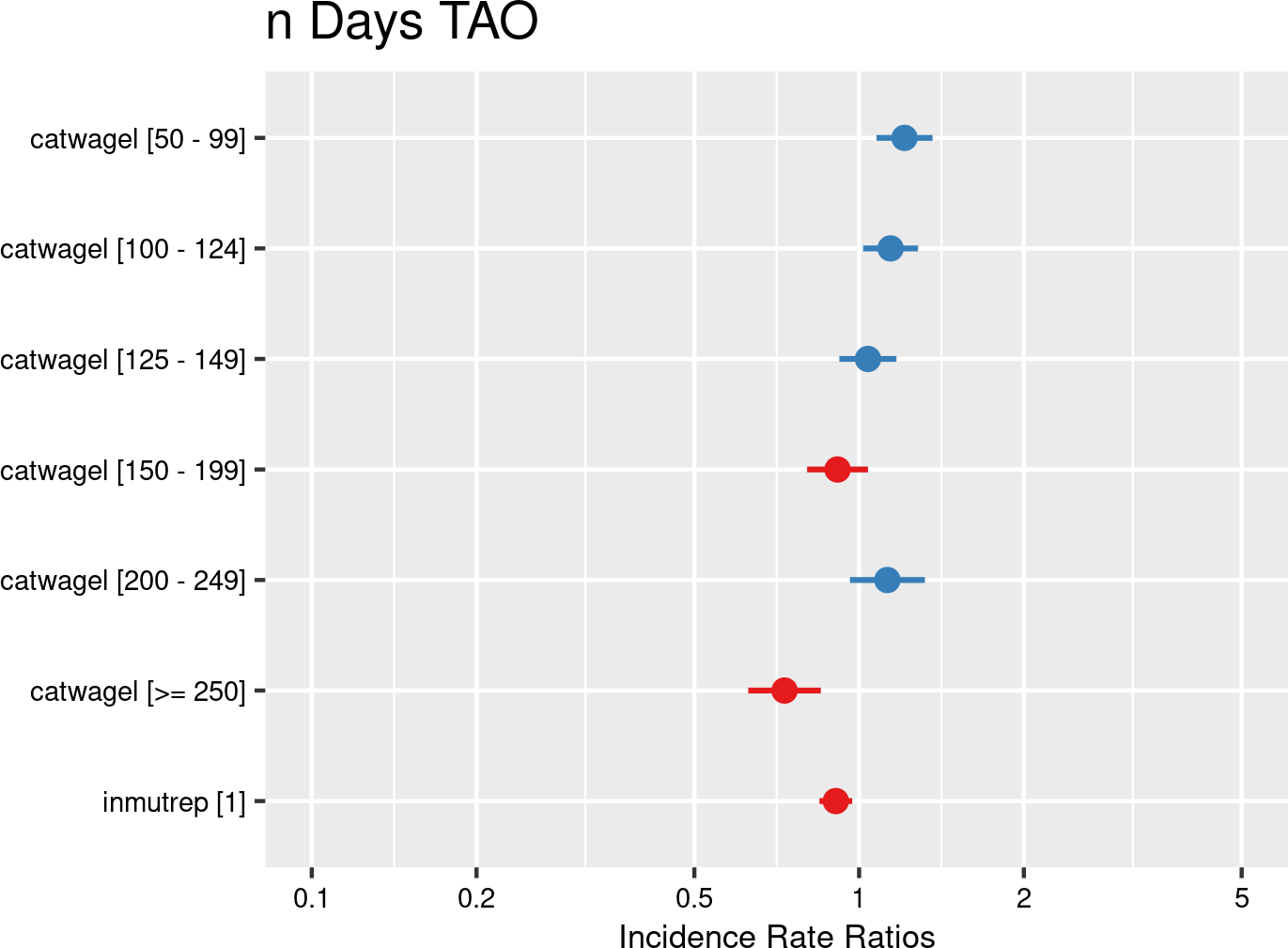

Wage categories were introduced as fixed effects, and companies and employees as random effects. The model is based on data of all mutual Liantis ESPP and PS customers. The model is adjusted for representativeness of the company (fixed effect inmutrep) regarding to sector, size and Flemish province.
As mentioned above, Figure 3.55 (a) and Figure 3.55 (b) are the results of the model assessing the relation between wage category and number of absenteeism days related to the workplace OA, based on the Liantis PS data. The results are somewhat different to these of the model above. The number of accepted days off increases significantly for a higher wage category: 27% more days for €200-249 wage category, while no significant results were found for the other categories. These inconsistent findings may be due to differences in the study populations between the Liantis PS data and the FEDRIS absenteeism data, the Liantis PS dataset being considerably smaller.
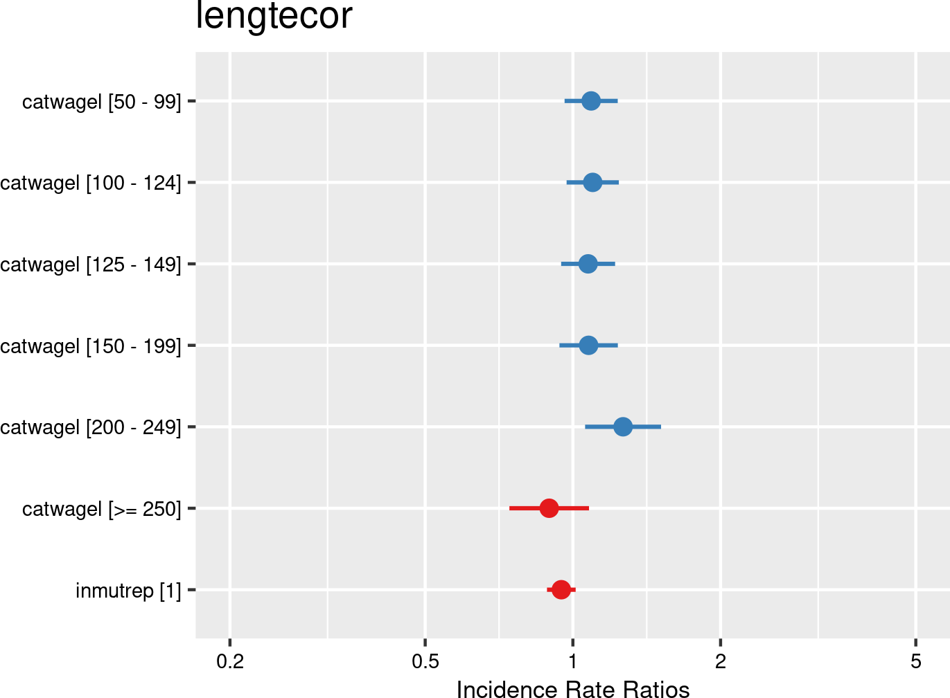

Wage categories were introduced as fixed effects, and companies and employees as random effects. The model is based on data of all mutual Liantis ESPP and PS customers. The model is adjusted for representativeness of the company (fixed effect inmutrep) regarding to sector, size and Flemish province.
Figure 3.56 (a) and Figure 3.56 (b) display the results of a model assessing the relationship between wage category and the direct wage cost of an OA. The results indicate that wage is a significant factor in determining the direct wage cost for an employer. How higher wage categories however, how smaller the cost in comparison with the reference. This is likely due to fewer and less serious accidents in the higher wage categories (when we compare with the results from the previous models).
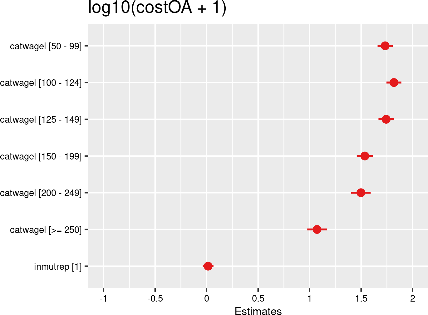

Wage categories were introduced as fixed effects, and companies and employees as random effects. The model is based on data of all mutual Liantis ESPP and PS customers. The model is adjusted for representativeness of the company (fixed effect inmutrep) regarding to sector, size and Flemish province.
The next 4 figures (Figure 3.57 (a) and Figure 3.57 (b), Figure 3.58 (a) and Figure 3.58 (b)) are displaying the results of a model assessing the relation between proportion of workers within a wage category and the severity degree of a company, which is again a variable at the company level. In the first model (Figure 3.57 (a) and Figure 3.57 (b)), validated number of absenteeism days from FEDRIS were used, while the second model (Figure 3.58 (a) and Figure 3.58 (b)) was based on the numbers of days off in the Liantis PS data. The initial figures indicate that a higher proportion of workers in three of the four lowest wage categories (<€50, €100-124, and €125-149) significantly increases the severity level within a company. However, the figures based on Liantis PS absenteeism data (Figure 3.58 (a) and Figure 3.58 (b)) show a slightly different pattern: a higher proportion of workers in all four lowest wage categories significantly increases the severity level within a company.
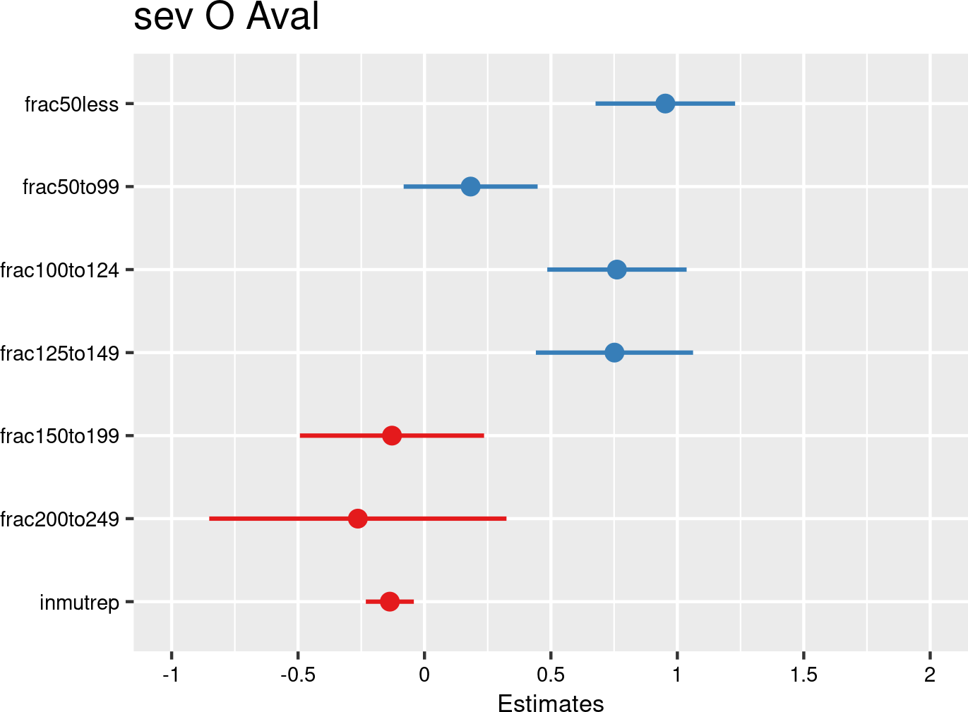

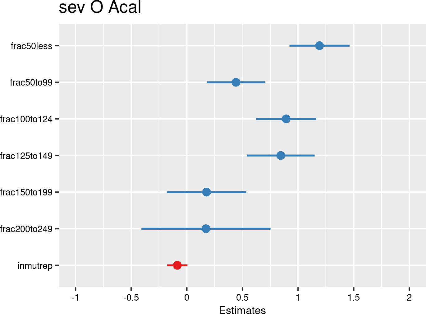

3.4.1.6 Residential location (province)
3.4.1.6.1 Descriptives
The NSSO provides data about the employee’s residence, including the province where they live. FEDRIS statistical reports offer the same information on residence: the province where the employee resides. From Liantis PS data, it’s possible to determine the employee’s province through their home address postal code. However, the notification unfortunately does not include the postal code of the employee’s residence. Since this information is missing in the notification passed to Liantis, the derived residential location of an employee experiencing an OA cannot be compared with the original notification’s residential location classification.
In the next 6 tables, an overview of all (accepted) OAs (Table 3.45 and Table 3.46), the commuting OAs (Table 3.47 and Table 3.48) and the workplace OAs (Table 3.49 and Table 3.50) are given.
In the first table ((Table 3.45, Table 3.47 and Table 3.49), the absolute numbers are provided stratified per province, next to the total number of employees, as available in the Liantis PS database.
In the second table (Table 3.46, Table 3.48 and Table 3.50), the relative numbers of the OAs per province are provided as percentages. In this tables, no information is available from the notifications.
From tables Table 3.46, Table 3.48, and Table 3.50, a number of observations can be made. We observe a discrepancy between NSSO and Liantis data: Liantis reports a significantly higher percentage of workers in West Flanders (43%) compared to NSSO figures (10%). In Limburg, East Flanders, and Flemish Brabant, the percentages are more consistent. For the other provinces, the proportion of Liantis workers is lower than the NSSO figures.
all accepted occupational accidents
| province | rszall | rszpriv | liaall | fedrisall | totalnot | totalnotmut | totalnotrepmutflan |
|---|---|---|---|---|---|---|---|
| Antwerpen | 25957449 | 20922766 | 2513258 | 246383 | NA | NA | NA |
| Brussel | 12692609 | 9885254 | 416523 | 80045 | NA | NA | NA |
| Henegouwen | 16060454 | 11302421 | 179155 | 129779 | NA | NA | NA |
| Limburg | 11871370 | 9248788 | 1343655 | 112247 | NA | NA | NA |
| Luik | 13448311 | 9263038 | 74145 | 120404 | NA | NA | NA |
| Luxemburg | 2671126 | 1671443 | 17809 | 19659 | NA | NA | NA |
| Namen | 6533638 | 4385366 | 60317 | 51896 | NA | NA | NA |
| Oost-Vlaanderen | 22366805 | 17033724 | 2441520 | 205517 | NA | NA | NA |
| Unknown | 3494077 | 3223122 | 1488183 | 59915 | NA | NA | NA |
| Vlaams Brabant | 16365498 | 12449407 | 1640213 | 115393 | NA | NA | NA |
| Waals Brabant | 5063215 | 3702801 | 73997 | 30005 | NA | NA | NA |
| West-Vlaanderen | 16643590 | 13273829 | 7807091 | 182134 | NA | NA | NA |
| province | percrszall | percrszpriv | percliaall | percfedrisall | perctotalnot | perctotalnotmut | perctotalnotrepmutflan |
|---|---|---|---|---|---|---|---|
| Antwerpen | 16.95 | 17.98 | 13.92 | 18.21 | NA | NA | NA |
| Brussel | 8.29 | 8.50 | 2.31 | 5.91 | NA | NA | NA |
| Henegouwen | 10.49 | 9.71 | 0.99 | 9.59 | NA | NA | NA |
| Limburg | 7.75 | 7.95 | 7.44 | 8.29 | NA | NA | NA |
| Luik | 8.78 | 7.96 | 0.41 | 8.90 | NA | NA | NA |
| Luxemburg | 1.74 | 1.44 | 0.10 | 1.45 | NA | NA | NA |
| Namen | 4.27 | 3.77 | 0.33 | 3.83 | NA | NA | NA |
| Oost-Vlaanderen | 14.60 | 14.64 | 13.52 | 15.19 | NA | NA | NA |
| Unknown | 2.28 | 2.77 | 8.24 | 4.43 | NA | NA | NA |
| Vlaams Brabant | 10.68 | 10.70 | 9.08 | 8.53 | NA | NA | NA |
| Waals Brabant | 3.31 | 3.18 | 0.41 | 2.22 | NA | NA | NA |
| West-Vlaanderen | 10.87 | 11.41 | 43.24 | 13.46 | NA | NA | NA |
commuting accepted occupational accidents
| province | rszall | rszpriv | liaall | fedrisall | totalnot | totalnotmut | totalnotrepmutflan |
|---|---|---|---|---|---|---|---|
| Antwerpen | 25957449 | 20922766 | 2513258 | 53566 | NA | NA | NA |
| Brussel | 12692609 | 9885254 | 416523 | 17193 | NA | NA | NA |
| Henegouwen | 16060454 | 11302421 | 179155 | 13749 | NA | NA | NA |
| Limburg | 11871370 | 9248788 | 1343655 | 18266 | NA | NA | NA |
| Luik | 13448311 | 9263038 | 74145 | 12266 | NA | NA | NA |
| Luxemburg | 2671126 | 1671443 | 17809 | 1846 | NA | NA | NA |
| Namen | 6533638 | 4385366 | 60317 | 6090 | NA | NA | NA |
| Oost-Vlaanderen | 22366805 | 17033724 | 2441520 | 39787 | NA | NA | NA |
| Unknown | 3494077 | 3223122 | 1488183 | 5201 | NA | NA | NA |
| Vlaams Brabant | 16365498 | 12449407 | 1640213 | 25839 | NA | NA | NA |
| Waals Brabant | 5063215 | 3702801 | 73997 | 5311 | NA | NA | NA |
| West-Vlaanderen | 16643590 | 13273829 | 7807091 | 27196 | NA | NA | NA |
| province | percrszall | percrszpriv | percliaall | percfedrisall | perctotalnot | perctotalnotmut | perctotalnotrepmutflan |
|---|---|---|---|---|---|---|---|
| Antwerpen | 16.95 | 17.98 | 13.92 | 23.67 | NA | NA | NA |
| Brussel | 8.29 | 8.50 | 2.31 | 7.60 | NA | NA | NA |
| Henegouwen | 10.49 | 9.71 | 0.99 | 6.08 | NA | NA | NA |
| Limburg | 7.75 | 7.95 | 7.44 | 8.07 | NA | NA | NA |
| Luik | 8.78 | 7.96 | 0.41 | 5.42 | NA | NA | NA |
| Luxemburg | 1.74 | 1.44 | 0.10 | 0.82 | NA | NA | NA |
| Namen | 4.27 | 3.77 | 0.33 | 2.69 | NA | NA | NA |
| Oost-Vlaanderen | 14.60 | 14.64 | 13.52 | 17.58 | NA | NA | NA |
| Unknown | 2.28 | 2.77 | 8.24 | 2.30 | NA | NA | NA |
| Vlaams Brabant | 10.68 | 10.70 | 9.08 | 11.42 | NA | NA | NA |
| Waals Brabant | 3.31 | 3.18 | 0.41 | 2.35 | NA | NA | NA |
| West-Vlaanderen | 10.87 | 11.41 | 43.24 | 12.02 | NA | NA | NA |
workplace accepted occupational accidents
| province | rszall | rszpriv | liaall | fedrisall | totalnot | totalnotmut | totalnotrepmutflan |
|---|---|---|---|---|---|---|---|
| Antwerpen | 25957449 | 20922766 | 2513258 | 192817 | NA | NA | NA |
| Brussel | 12692609 | 9885254 | 416523 | 62852 | NA | NA | NA |
| Henegouwen | 16060454 | 11302421 | 179155 | 116030 | NA | NA | NA |
| Limburg | 11871370 | 9248788 | 1343655 | 93981 | NA | NA | NA |
| Luik | 13448311 | 9263038 | 74145 | 108138 | NA | NA | NA |
| Luxemburg | 2671126 | 1671443 | 17809 | 17813 | NA | NA | NA |
| Namen | 6533638 | 4385366 | 60317 | 45806 | NA | NA | NA |
| Oost-Vlaanderen | 22366805 | 17033724 | 2441520 | 165730 | NA | NA | NA |
| Unknown | 3494077 | 3223122 | 1488183 | 54714 | NA | NA | NA |
| Vlaams Brabant | 16365498 | 12449407 | 1640213 | 89554 | NA | NA | NA |
| Waals Brabant | 5063215 | 3702801 | 73997 | 24694 | NA | NA | NA |
| West-Vlaanderen | 16643590 | 13273829 | 7807091 | 154938 | NA | NA | NA |
| province | percrszall | percrszpriv | percliaall | percfedrisall | perctotalnot | perctotalnotmut | perctotalnotrepmutflan |
|---|---|---|---|---|---|---|---|
| Antwerpen | 16.95 | 17.98 | 13.92 | 17.11 | NA | NA | NA |
| Brussel | 8.29 | 8.50 | 2.31 | 5.58 | NA | NA | NA |
| Henegouwen | 10.49 | 9.71 | 0.99 | 10.29 | NA | NA | NA |
| Limburg | 7.75 | 7.95 | 7.44 | 8.34 | NA | NA | NA |
| Luik | 8.78 | 7.96 | 0.41 | 9.59 | NA | NA | NA |
| Luxemburg | 1.74 | 1.44 | 0.10 | 1.58 | NA | NA | NA |
| Namen | 4.27 | 3.77 | 0.33 | 4.06 | NA | NA | NA |
| Oost-Vlaanderen | 14.60 | 14.64 | 13.52 | 14.70 | NA | NA | NA |
| Unknown | 2.28 | 2.77 | 8.24 | 4.85 | NA | NA | NA |
| Vlaams Brabant | 10.68 | 10.70 | 9.08 | 7.95 | NA | NA | NA |
| Waals Brabant | 3.31 | 3.18 | 0.41 | 2.19 | NA | NA | NA |
| West-Vlaanderen | 10.87 | 11.41 | 43.24 | 13.75 | NA | NA | NA |
3.4.1.6.2 Models
The following Table 3.51 table summarizes the results of the models assessing the relationship between residential location categories and the several outcomes related to OAs. Below the table, details are provided about the data used for the analyses. The results of the nine models are then presented both graphically and in a table.
| catresiloc | chance to notify | chance on refusal | chance commuting | chance workplace | freq degree | chance serious | nDays TAO V/C | cost | sev degree V/C |
|---|---|---|---|---|---|---|---|---|---|
| Antwerp | REF | REF | REF | REF | ns | REF | REF | REF | ns |
| Brussel | < | ns | ns | < | < | ns | >/> | > | ns |
| Hainaut | > | ns | ns | > | > | ns | ns | ns | ns |
| Limburg | < | ns | ns | < | < | ns | >/ns | ns | ns |
| Liège | ns | ns | ns | ns | ns | ns | ns | > | ns |
| Luxembourg | > | ns | ns | > | ns | ns | ns | ns | ns |
| Namur | ns | ns | ns | ns | ns | ns | ns | ns | ns |
| East Fl | > | ns | ns | ns | ns | ns | ns | ns | ns |
| Fl Brabant | < | ns | ns | < | ns | ns | >/> | ns | ns |
| Wal Brabant | ns | ns | ns | ns | ns | ns | ns/> | ns | ns |
| West-Fl | > | ns | > | > | > | ns | ns | ns | ns |
| occur | accept | occur | occur | occur | severe | severe | severe | severe | |
| empl | empl | empl | empl | comp | empl | empl | empl | comp | |
| c/w all | c/w ref | c acc | w acc | w acc | w acc | w acc | w acc | w acc |
- occur: data include all workers, chance for occurrence is calculated for the outcome
- accept: data include only workers with a notification of OA
- severe: data include only workers with an accepted OA
- c/w all: commuting and workplace accidents, including refused and accidents without decisions
- c/w ref: accepted or refused commuting and workplace accidents
- c acc: accepted commuting accidents
- w acc: accepted workplace accidents
- empl: the outcome is situated at the individual level
- comp: the outcome is situated at the company level
- nDaysTAO: number of days absenteeism related to the OA
- V/C: Validated number of days (available from FEDRIS) / Calculated number of days (based on the Liantis PS data)
Residential location (province) and occupational accidents
- Workers residing in West-Flanders, Luxembourg, and Hainaut have a significantly higher likelihood of reporting occupational accidents and experiencing occupational workplace accidents compared to those living in Antwerp
- The province in which an employee is living does not significantly determine the likelihood to have an accepted commuting occupational accident.
- The figures suggest that workers who are living in Brussels and Flemish Brabant have a higher number of absenteeism days due to occupational accidents.
- The findings suggest that workers living in Brussel have a significant higher direct wage cost related to the occupational accident, for employers in comparison with the direct wage cost of workers living in Antwerp.
- The proportion of workers living in West-Flanders and Hainaut significantly increases the frequency degree (but not the severity degree) of occupational accidents within a company.
According to Figure 3.59 (a) and Figure 3.59 (b), workers residing in Luxembourg, West-Flanders and Hainaut have a significantly higher likelihood of reporting OAs (both commuting and workplace accidents) compared to those living in Antwerp, even after accounting for differences in company representativeness (link to methodology).
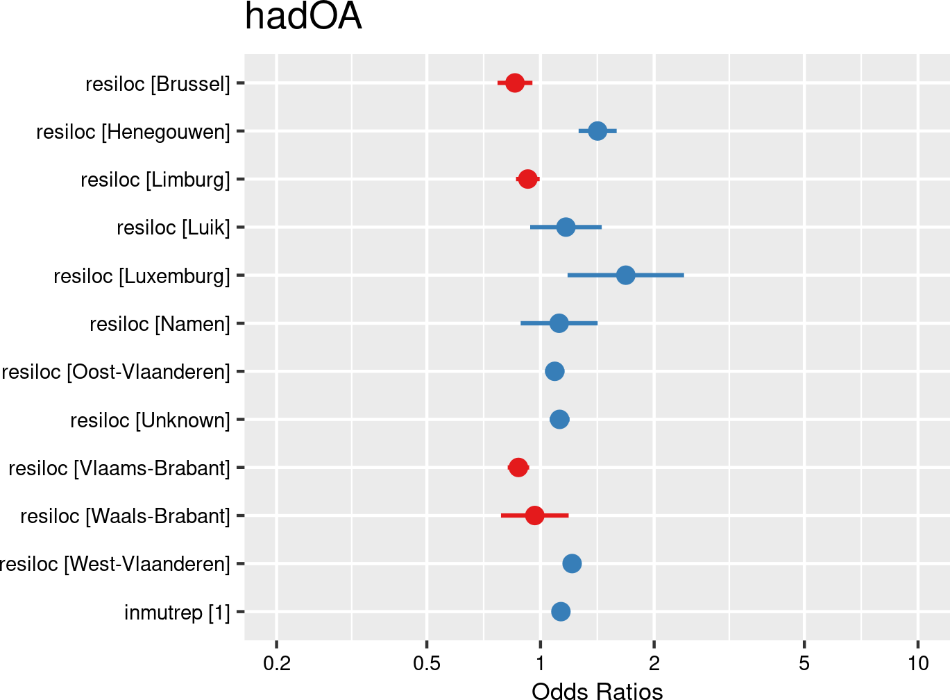

Residential location categories (provinces) were introduced as fixed effects, and companies and employees as random effects. The model is based on data from employees with and without OAs from all mutual Liantis ESPP and PS customers. The model is adjusted for representativeness of the company (fixed effect inmutrep) regarding to sector, size and Flemish province.
According to Figure 3.60 (a) and Figure 3.60 (b), the province in which a worker lives does not significantly determine the likelihood of a reported OA being rejected by the insurer.
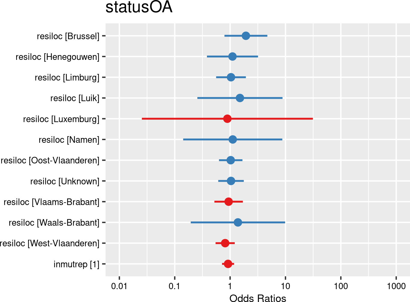

Residential location categories (provinces) were introduced as fixed effects, and companies and employees as random effects. The model is based on data from employees notifying OAs from all mutual Liantis ESPP and PS customers. The model is adjusted for representativeness of the company (fixed effect inmutrep) regarding to sector, size and Flemish province.
According to Figure 3.61 (a) and Figure 3.61 (b), the province in which an employee is living does not significantly determine the likelihood to have an accepted commuting accident.


Residential location categories (provinces) were introduced as fixed effects, and companies and employees as random effects. The model is based on data from employees with and without OAs from all mutual Liantis ESPP and PS customers. The model is adjusted for representativeness of the company (fixed effect inmutrep) regarding to sector, size and Flemish province.
Figure 3.62 (a) and Figure 3.62 (b) show the estimates for the relation between residence (province) and an accepted workplace OA. The results indicate that workers living in West-Flanders, Hainout and Luxembourg have a significantly higher likelihood of having an accepted workplace OA.
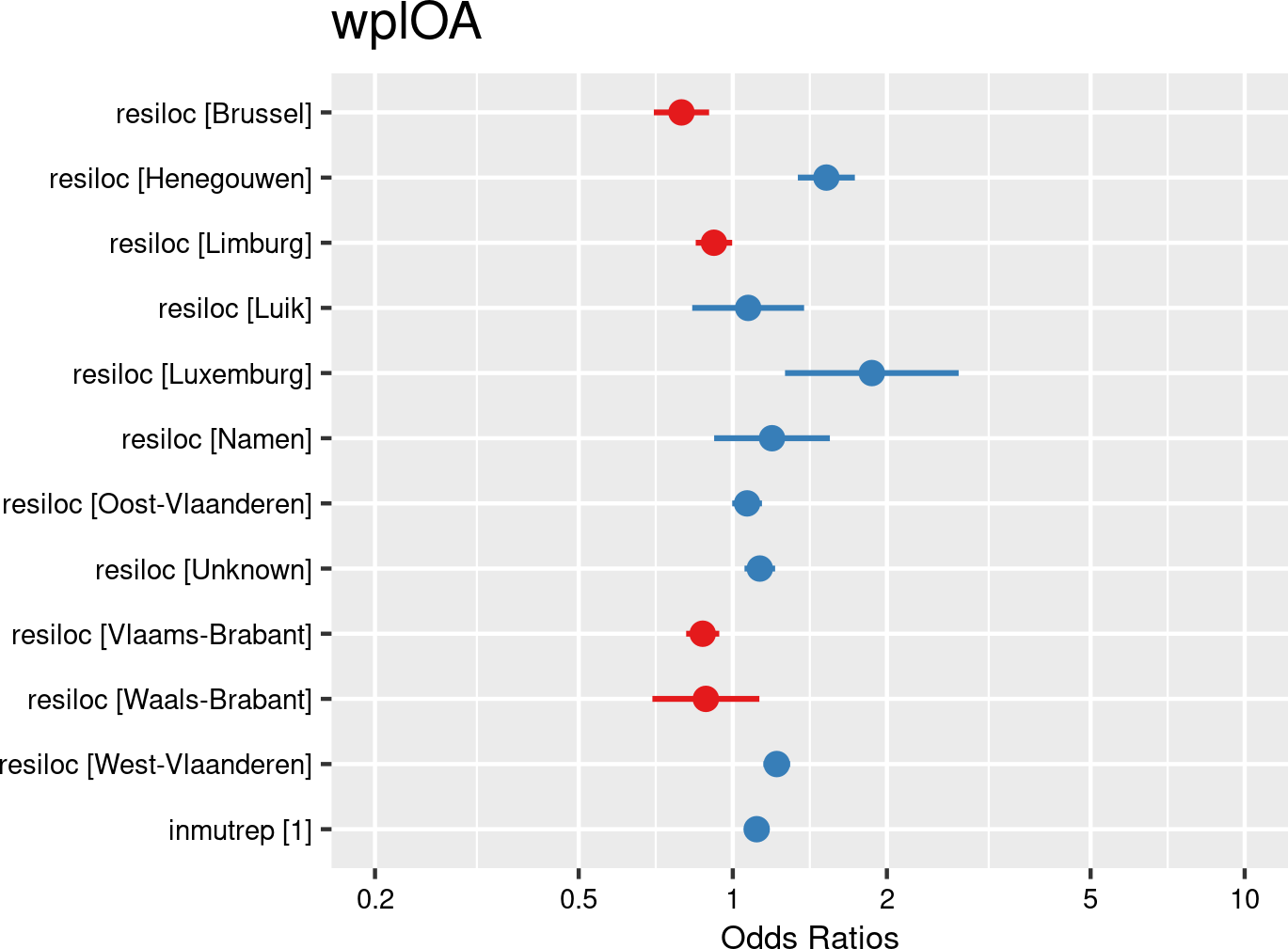

Residence categories (provinces) were introduced as fixed effects, and companies and employees as random effects. The model is based on data from employees with and without OAs from all mutual Liantis ESPP and PS customers. The model is adjusted for representativeness of the company (fixed effect inmutrep) regarding to sector, size and Flemish province.
Figure 3.63 (a) and Figure 3.63 (b) present a model estimating the frequency degree of OAs at the company level, contrasting with previous models that focused on individual employee accident probabilities. These figures show that a higher proportion of workers living in West-Flanders and Hainaut significantly increases the frequency degree of OAs within a company. On the contrary, a higher proportion workers from Limbourg and Brussels, significantly decreases the frequency degree of a company.
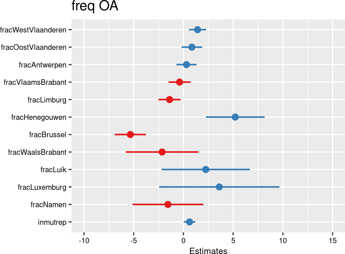

Residential location categories (provinces) proportions were introduced as fixed effects, and companies as random effects. The model is based on data of all mutual Liantis ESPP and PS customers. The model is adjusted for representativeness of the company (fixed effect inmutrep) regarding to sector, size and Flemish province.
Figure 3.64 (a) and Figure 3.64 (b) present a model estimating the likelihood of an accepted accident being classified as serious according to Belgian law. These figures indicate that the province a worker is living in does not significantly determine the likelihood an OA is classified as serious.
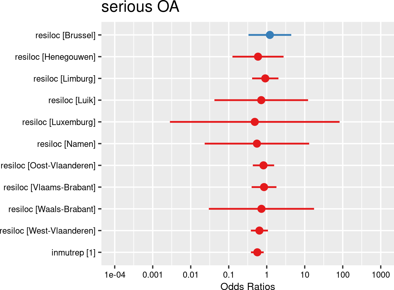

Residential location categories (provinces) were introduced as fixed effects, and companies and employees as random effects. The model is based on data of all mutual Liantis ESPP and PS customers. The model is adjusted for representativeness of the company (fixed effect inmutrep) regarding to sector, size and Flemish province.
Figure 3.65 (a) and Figure 3.65 (b) show the results of a model assessing the relationship between residence and the number of absenteeism days. These figures are based on absenteeism data from FEDRIS, while Figure 3.66 (a) and Figure 3.66 (b) present the same model using data from Liantis PS. The figures indicate that workers who are living in Brussels, Flemish Brabant or Limbourg have a higher validated number of absenteeism days due to OAs. The number of accepted days off increases significantly for workers in Brussels, Flemish Brabant and Limbourg, with respectively 66%, 15% and 21% in comparison with workers living in Antwerp.
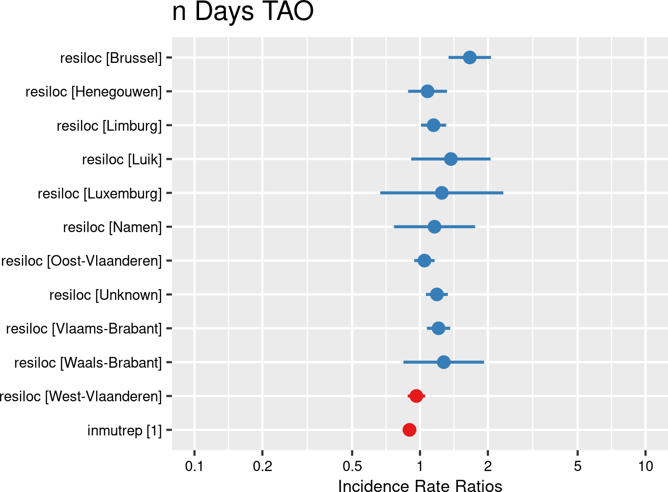

Residential location categories (provinces) were introduced as fixed effects, and companies and employees as random effects. The model is based on data of all mutual Liantis ESPP and PS customers. The model is adjusted for representativeness of the company (fixed effect inmutrep) regarding to sector, size and Flemish province.
As mentioned above, Figure 3.66 (a) and Figure 3.66 (b) are the results of the model assessing the relation between residence and the number of absenteeism days related to the workplace accident, based on the Liantis PS data. The findings are more or less in line with those of the model based on the FEDRIS absenteeism data: workers living in Brussels and Flemish Brabant have more absenteeism days related to OAs then workers from Antwerp. However, in this sample, also workers from Walloon Brabant have a significant higher number of absenteeism days (61%) related to OAs in comparison with workers from Antwerp.
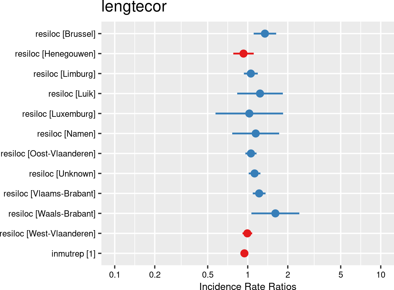

Residential location categories (provinces) were introduced as fixed effects, and companies and employees as random effects. The model is based on data of all mutual Liantis ESPP and PS customers. The model is adjusted for representativeness of the company (fixed effect inmutrep) regarding to sector, size and Flemish province.
Figure 3.67 (a) and Figure 3.67 (b) show the results of a model evaluating the relationship between residence and the direct wage cost of an OA. The findings indicate that workers living in Brussels have a significant higher direct wage cost related to the OA, for employers in comparison with the direct wage cost of workers living in Antwerp.
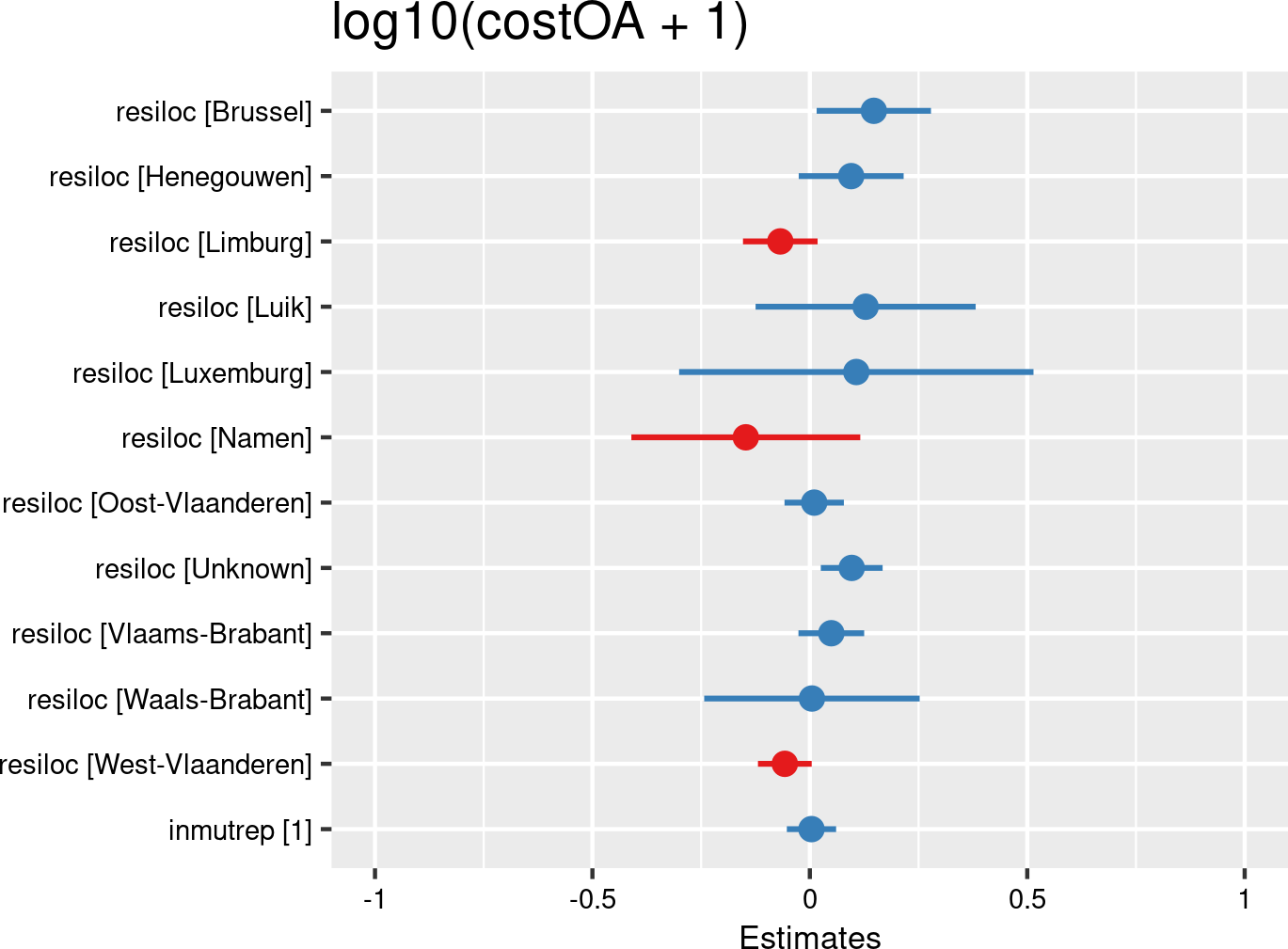

Residential location categories (provinces) were introduced as fixed effects, and companies and employees as random effects. The model is based on data of all mutual Liantis ESPP and PS customers. The model is adjusted for representativeness of the company (fixed effect inmutrep) regarding to sector, size and Flemish province.
The next 4 figures (Figure 3.68 (a) and Figure 3.68 (b), Figure 3.69 (a) and Figure 3.69 (b)) are displaying the results of a model assessing the relation between proportion of workers living within a province and the severity degree of a company, which is again a variable at the company level. In the first model (Figure 3.68 (a) and Figure 3.68 (b)), validated number of absenteeism days from FEDRIS were used, while the second model Figure 3.69 (a) and Figure 3.69 (b)) was based on the numbers of days off in the Liantis PS data. The results of both models indicate that the proportion of workers living in a particular province does not determine the severity level within a company.


Residential location category (province) proportions were introduced as fixed effects, and companies as random effects. The model is based on data of all mutual Liantis ESPP and PS customers. The model is adjusted for representativeness of the company (fixed effect inmutrep) regarding to sector, size and Flemish province.
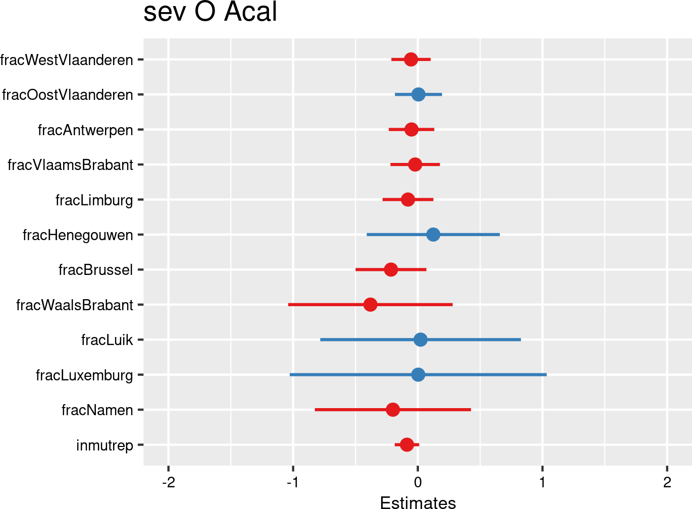

Residential location category (province) proportions were introduced as fixed effects, and companies as random effects. The model is based on data of all mutual Liantis ESPP and PS customers. The model is adjusted for representativeness of the company (fixed effect inmutrep) regarding to sector, size and Flemish province.
3.4.1.7 Commuting distance
3.4.1.7.1 Descriptives
NSSO nor FEDRIS provide statistics on commuting distance. From Liantis PS data however, it also possible to roughly estimate the commuting distance of a worker by calculating the distance between the residential location and the postal code of the employer.
From the tables Table 3.53, Table 3.55 and Table 3.57, some important findings can be noticed. Employees commuting 10–19 km have the highest probability of experiencing an OA (both commuting and workplace accidents), those commuting 5–9 km have the lowest probability. Interestingly, the shortest (<5 km) and longest (\(\geq\) 20 km) commutes are associated with moderate accident probabilities. This suggests that medium-range commuters (10–19 km) might be at greater risk, possibly due to factors like higher traffic exposure or fatigue without the compensating benefits of very short or very long commutes (e.g., more cautious behaviour or different transport modes).
all accepted occupational accidents
| catdist | rszall | rszpriv | liaall | fedrisall | totalnot | totalnotmut | totalnotrepmutflan |
|---|---|---|---|---|---|---|---|
| <5 km | NA | NA | 5946135 | NA | 11236 | 11236 | 4643 |
| 5 - 9 km | NA | NA | 2592608 | NA | 6743 | 6743 | 2917 |
| 10 - 19 km | NA | NA | 4006374 | NA | 11655 | 11655 | 5317 |
| >=20 km | NA | NA | 3964647 | NA | 10600 | 10600 | 5194 |
| NA | NA | NA | 1546102 | NA | 154985 | 21001 | 7959 |
| catdist | percrszall | percrszpriv | percliaall | percfedrisall | perctotalnot | perctotalnotmut | perctotalnotrepmutflan |
|---|---|---|---|---|---|---|---|
| <5 km | NA | NA | 36.0 | NA | 27.9 | 27.9 | 25.7 |
| 5 - 9 km | NA | NA | 15.7 | NA | 16.8 | 16.8 | 16.1 |
| 10 - 19 km | NA | NA | 24.3 | NA | 29.0 | 29.0 | 29.4 |
| >=20 km | NA | NA | 24.0 | NA | 26.3 | 26.3 | 28.7 |
| NA | NA | NA | NA | NA | NA | NA | NA |
commuting accepted occupational accidents
| catdist | rszall | rszpriv | liaall | fedrisall | totalnot | totalnotmut | totalnotrepmutflan |
|---|---|---|---|---|---|---|---|
| <5 km | NA | NA | 5946135 | NA | 1484 | 1484 | 674 |
| 5 - 9 km | NA | NA | 2592608 | NA | 972 | 972 | 473 |
| 10 - 19 km | NA | NA | 4006374 | NA | 1561 | 1561 | 849 |
| >=20 km | NA | NA | 3964647 | NA | 1675 | 1675 | 853 |
| NA | NA | NA | 1546102 | NA | 22695 | 2907 | 1263 |
| catdist | percrszall | percrszpriv | percliaall | percfedrisall | perctotalnot | perctotalnotmut | perctotalnotrepmutflan |
|---|---|---|---|---|---|---|---|
| <5 km | NA | NA | 36.0 | NA | 26.1 | 26.1 | 23.7 |
| 5 - 9 km | NA | NA | 15.7 | NA | 17.1 | 17.1 | 16.6 |
| 10 - 19 km | NA | NA | 24.3 | NA | 27.4 | 27.4 | 29.8 |
| >=20 km | NA | NA | 24.0 | NA | 29.4 | 29.4 | 29.9 |
| NA | NA | NA | NA | NA | NA | NA | NA |
workplace accepted occupational accidents
| catdist | rszall | rszpriv | liaall | fedrisall | totalnot | totalnotmut | totalnotrepmutflan |
|---|---|---|---|---|---|---|---|
| <5 km | NA | NA | 5946135 | NA | 9752 | 9752 | 3969 |
| 5 - 9 km | NA | NA | 2592608 | NA | 5771 | 5771 | 2444 |
| 10 - 19 km | NA | NA | 4006374 | NA | 10094 | 10094 | 4468 |
| >=20 km | NA | NA | 3964647 | NA | 8925 | 8925 | 4341 |
| NA | NA | NA | 1546102 | NA | 132290 | 18094 | 6696 |
| catdist | percrszall | percrszpriv | percliaall | percfedrisall | perctotalnot | perctotalnotmut | perctotalnotrepmutflan |
|---|---|---|---|---|---|---|---|
| <5 km | NA | NA | 36.0 | NA | 28.2 | 28.2 | 26.1 |
| 5 - 9 km | NA | NA | 15.7 | NA | 16.7 | 16.7 | 16.1 |
| 10 - 19 km | NA | NA | 24.3 | NA | 29.2 | 29.2 | 29.4 |
| >=20 km | NA | NA | 24.0 | NA | 25.8 | 25.8 | 28.5 |
| NA | NA | NA | NA | NA | NA | NA | NA |
3.4.1.7.2 Models
The following Table 3.58 table summarizes the results of the models assessing the relationship between commuting distance categories and the several outcomes related to OAs. Below the table, details are provided about the data used for the analyses. The results of the nine models are then presented both graphically and in a table.
| catdist | chance to notify | chance on refusal | chance commuting | chance workplace | freq degree | chance serious | nDays TAO V/C | cost | sev degree V/C |
|---|---|---|---|---|---|---|---|---|---|
| less than 5 | REF | REF | REF | REF | < | REF | REF | REF | </ns |
| 5 to 9 | > | ns | > | > | > | ns | ns | > | ns |
| 10 to 19 | > | ns | > | > | > | ns | ns | ns | ns |
| 20 and more | > | ns | > | > | > | ns | ns | > | ns/< |
| occur | accept | occur | occur | occur | severe | severe | severe | severe | |
| empl | empl | empl | empl | comp | empl | empl | empl | comp | |
| c/w all | c/w ref | c acc | w acc | w acc | w acc | w acc | w acc | w acc |
- occur: data include all workers, chance for occurrence is calculated for the outcome
- accept: data include only workers with a notification of OA
- severe: data include only workers with an accepted OA
- c/w all: commuting and workplace accidents, including refused and accidents without decisions
- c/w ref: accepted or refused commuting and workplace accidents
- c acc: accepted commuting accidents
- w acc: accepted workplace accidents
- empl: the outcome is situated at the individual level
- comp: the outcome is situated at the company level
- nDaysTAO: number of days absenteeism related to the OA
- V/C: Validated number of days (available from FEDRIS) / Calculated number of days (based on the Liantis PS data)
Commuting distance and occupational accidents
- Workers with commuting distances of 5 km and more all have higher chances to report occupational accidents (commuting and workplace accidents) compared to those living less than 5 km from work.
- Odds for accepted commuting occupational accidents show an increasing trend for larger commuting distance categories.
- Workers working between 10 and 20 km from home show the highest odds to experience an accepted workplace accident. A multivariable model should confirm this finding whether commuting distances do not only impact the chance to experience commuting accidents, but as well the chance to experience workplace accidents.
- Higher proportions of workers working more than 5 km from home significantly increase the frequency degree of a company while a higher proportion of workers working less than 5 km from home significantly decreases it.
- Commuting distance categories do not do not significantly determine whether an occupational accident is classified as serious nor the number of absenteeism days due to occupational accidents.
- All commuting distance categories of 5 and more km show a significant higher direct wage cost than the reference category.
- Severity degrees tend to be lower for companies with higher proportions of workers in the commuting distance categories less than 5 and 20 and more km.
Figure 3.70 (a) and Figure 3.70 (b) show that people working 5 and more km from home have a higher chance to report an OA. People from the category 10 - 19 km have a 34% higher chance compared to the reference category.
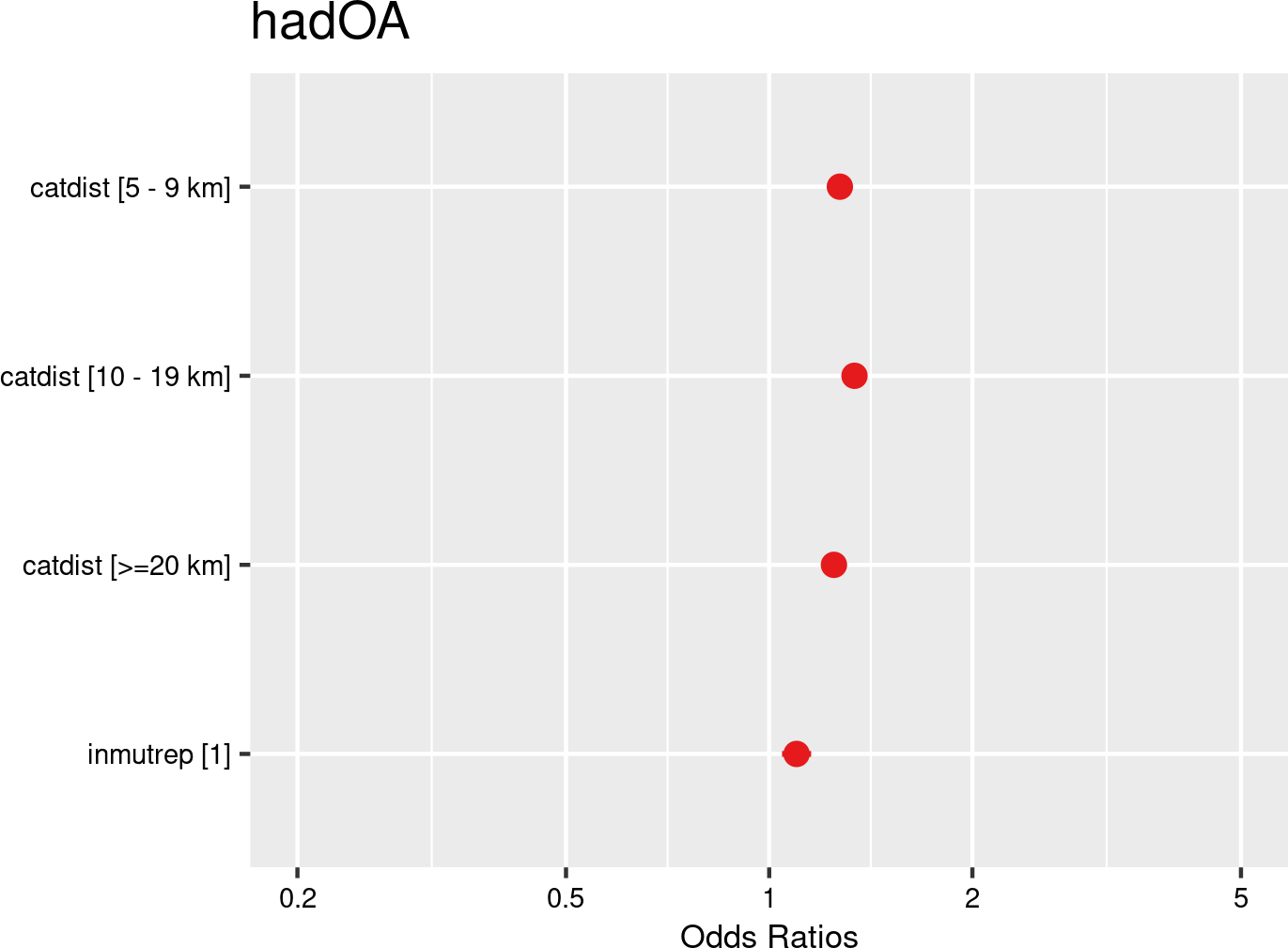

Commuting distance categories were introduced as fixed effects, and companies and employees as random effects. The model is based on data from employees with and without OAs from all mutual Liantis ESPP and PS customers. The model is adjusted for representativeness of the company (fixed effect inmutrep) regarding to sector, size and Flemish province.
According to Figure 3.71 (a) and Figure 3.71 (b), the distance category between the residential and workplace location does not significantly determine the likelihood of a reported OA being rejected by the insurer.
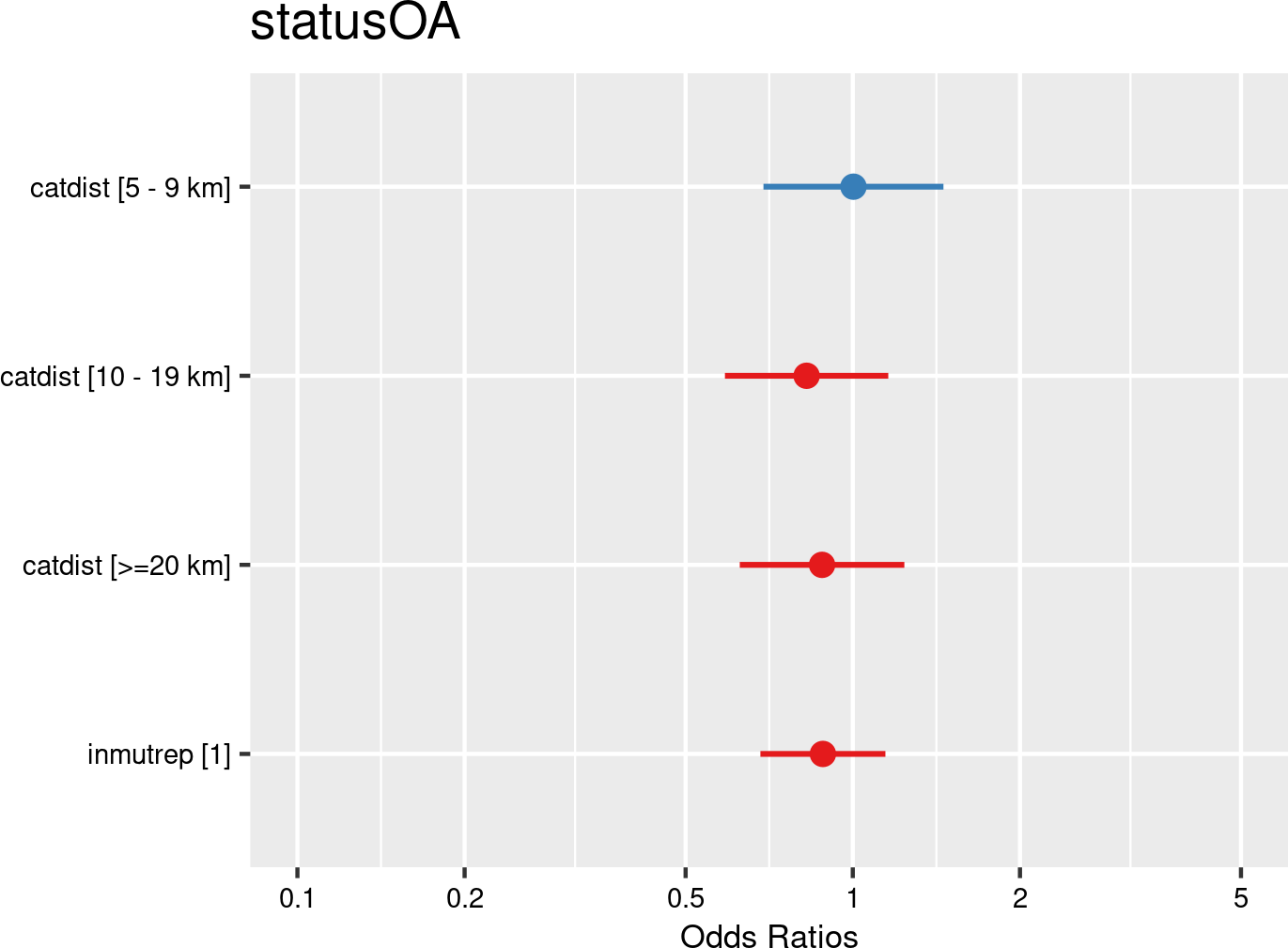

Commuting distance categories were introduced as fixed effects, and companies and employees as random effects. The model is based on data from employees notifying OAs from all mutual Liantis ESPP and PS customers. The model is adjusted for representativeness of the company (fixed effect inmutrep) regarding to sector, size and Flemish province.
According to Figure 3.72 (a) and Figure 3.72 (b), the commuting distance category significantly determines the likelihood to have an accepted commuting accident. Workers falling into categories of 5 km and more show higher odds for commuting accidents with a trend for higher odds for longer distances. While the increasing trend is in line with the findings of (Ponsin et al., 2020), the relative differences between the categories are not of the same order of magnitude (we find 50% and not 400% more chance for commuting distances \(\geq\) 20 km). We do not have any information on the perception of the risk nor the mode of transport (by bicycle, on foot, by car,…) and thus cannot compare or results with other studies (Fadzil & Bulgiba, 2023; Finnish Institute of Occupational Health, 2025).
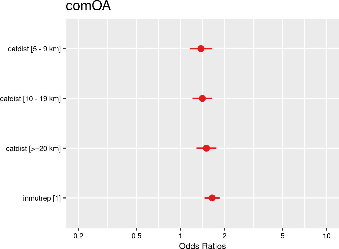

Commuting distance categories were introduced as fixed effects, and companies and employees as random effects. The model is based on data from employees with and without OAs from all mutual Liantis ESPP and PS customers. The model is adjusted for representativeness of the company (fixed effect inmutrep) regarding to sector, size and Flemish province.
Figure 3.73 (a) and Figure 3.73 (b) show that the commuting distance category significantly determines the likelihood to experience an accepted workplace accident. Workers falling into categories of 5 km and more show higher odds for workplace accidents with the highest ratio (35% higher) occurring in the category 10 - 19 km.
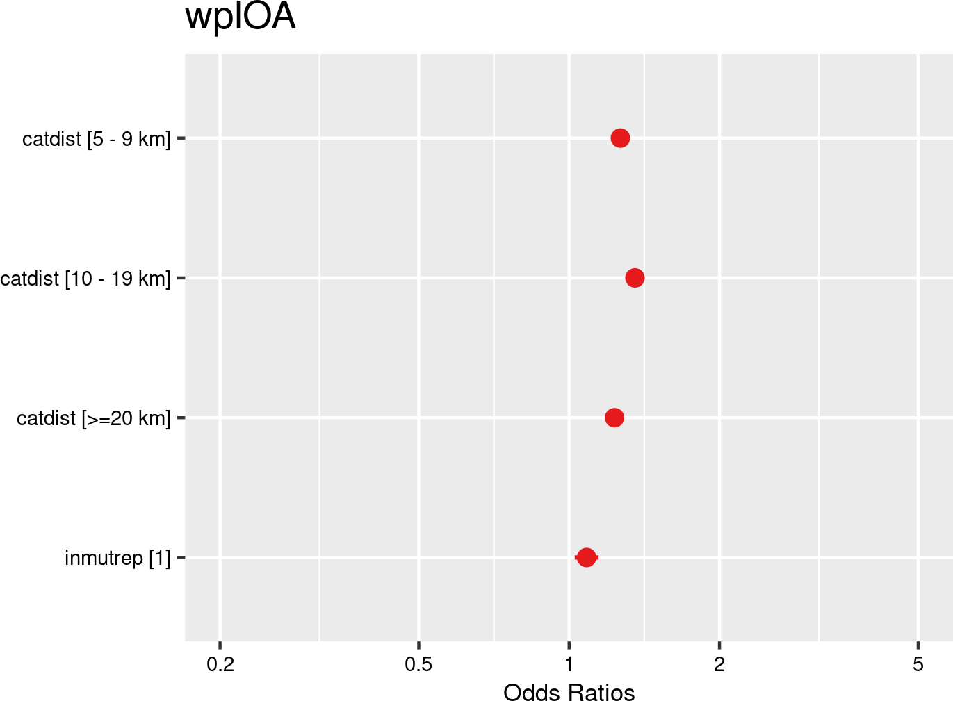

Commuting distance categories were introduced as fixed effects, and companies and employees as random effects. The model is based on data from employees with and without OAs from all mutual Liantis ESPP and PS customers. The model is adjusted for representativeness of the company (fixed effect inmutrep) regarding to sector, size and Flemish province.
Figure 3.74 (a) and Figure 3.74 (b) present a model estimating the frequency degree of OAs at the company level, contrasting with previous models that focused on the individual employee accident probabilities. These figures show that a higher proportion of workers living between ten and twenty km from work significantly increases the frequency degree of OAs within a company. On the contrary, a higher proportion workers living less than 5 km from work, significantly decreases the frequency degree of a company.
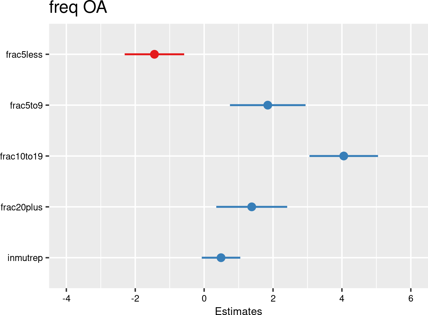

Commuting distance categories proportions were introduced as fixed effects, and companies as random effects. The model is based on data of all mutual Liantis ESPP and PS customers. The model is adjusted for representativeness of the company (fixed effect inmutrep) regarding to sector, size and Flemish province.
Figure 3.75 (a) and Figure 3.75 (b) present a model estimating the likelihood of an accepted accident being classified as serious according to Belgian law. These figures indicate that the commuting distance category does not significantly determine the likelihood an OA is classified as serious.
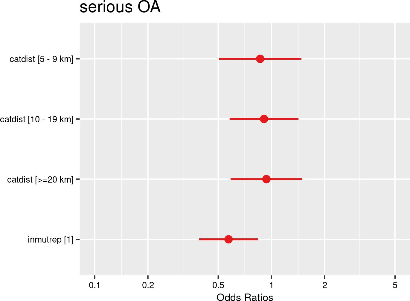

Commuting distance categories were introduced as fixed effects, and companies and employees as random effects. The model is based on data of all mutual Liantis ESPP and PS customers. The model is adjusted for representativeness of the company (fixed effect inmutrep) regarding to sector, size and Flemish province.
Figure 3.76 (a) and Figure 3.76 (b) show the results of a model assessing the relationship between commuting distance categories and absenteeism days. These figures are based on absenteeism data FEDRIS, while Figure 3.77 (a) and Figure 3.77 (b) present the same model using data from Liantis PS. The figures indicate that the commuting distance category of a worker does not significantly determine the number of days the worker is absent after experiencing an accepted workplace accident.
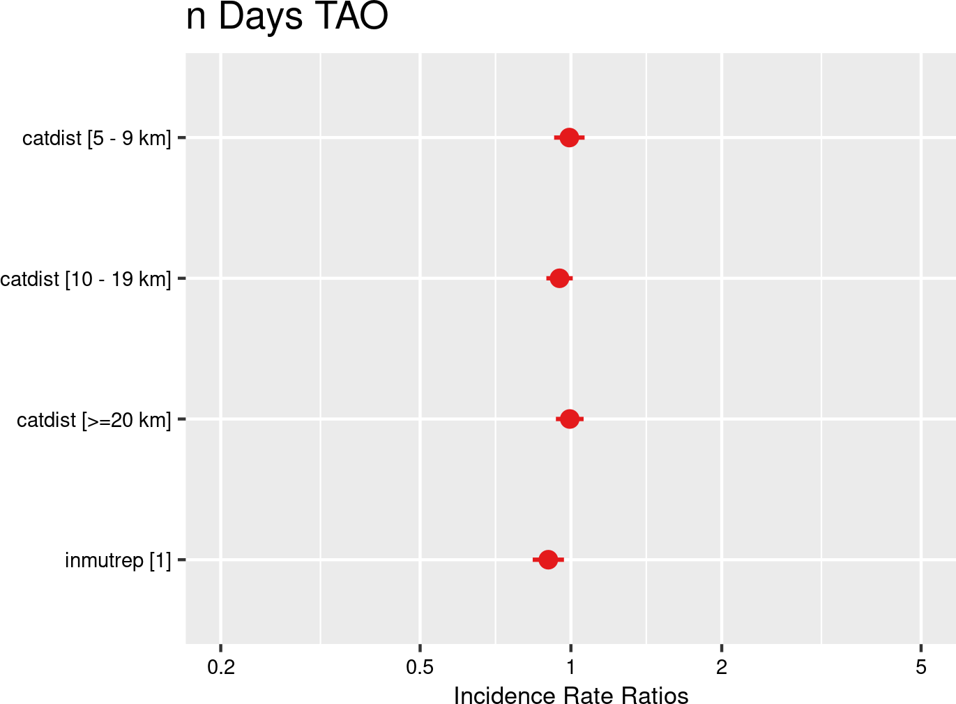

Commuting distance categories were introduced as fixed effects, and companies and employees as random effects. The model is based on data of all mutual Liantis ESPP and PS customers. The model is adjusted for representativeness of the company (fixed effect inmutrep) regarding to sector, size and Flemish province.
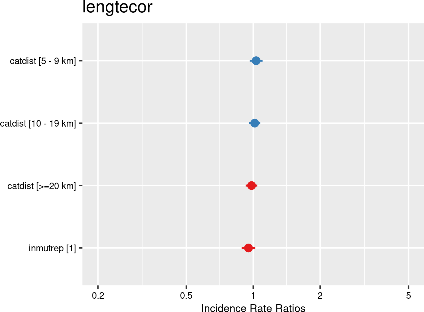

Commuting distance categories were introduced as fixed effects, and companies and employees as random effects. The model is based on data of all mutual Liantis ESPP and PS customers. The model is adjusted for representativeness of the company (fixed effect inmutrep) regarding to sector, size and Flemish province.
Figure 3.78 (a) and Figure 3.78 (b) show the results of a model evaluating the relationship between commuting distance category and the direct wage cost of an OA. The findings indicate that workers living 5-9 and 20 and more km away from their workplace have a significant higher direct wage cost related to the OA that workers from the reference category living less than 5 km from their workplace.
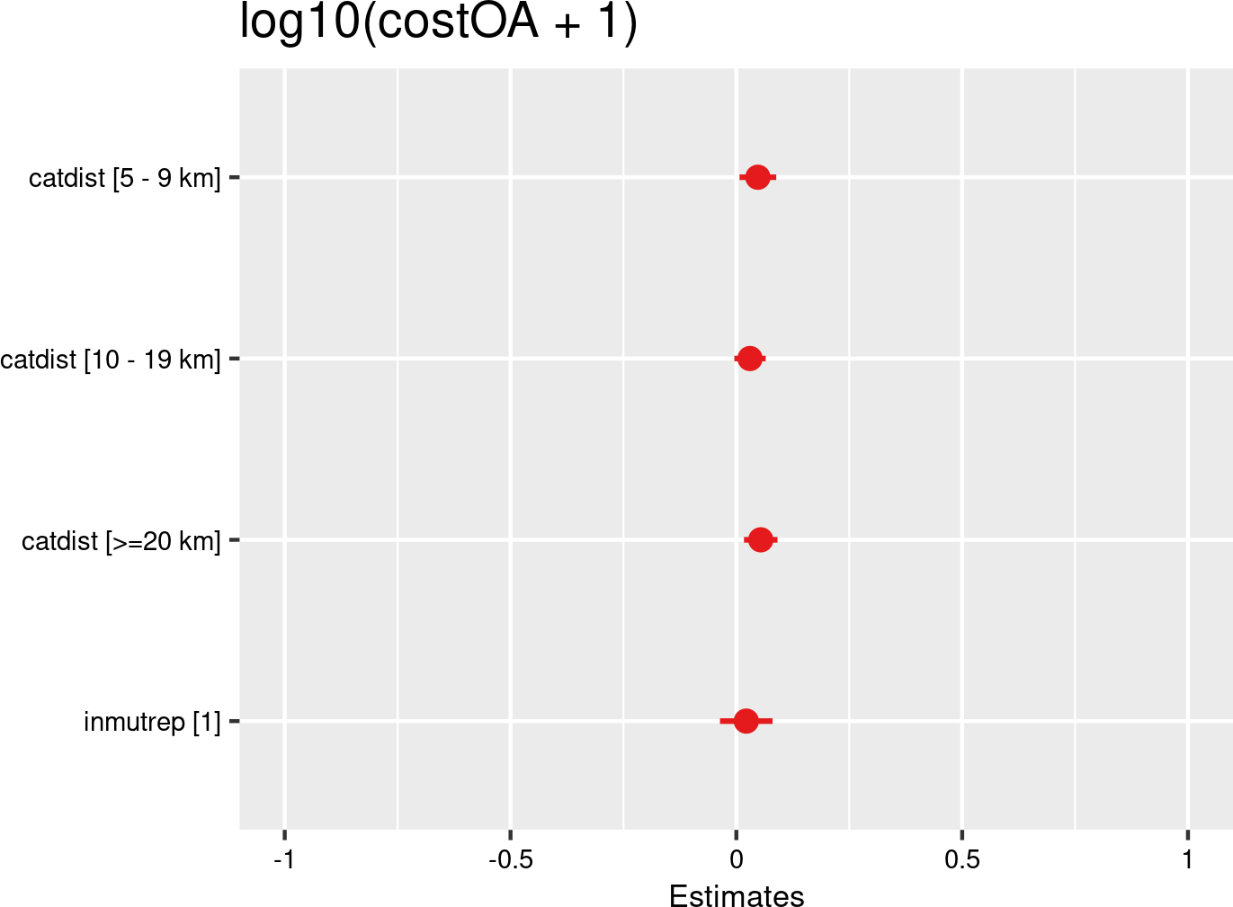

Commuting distance categories were introduced as fixed effects, and companies and employees as random effects. The model is based on data of all mutual Liantis ESPP and PS customers. The model is adjusted for representativeness of the company (fixed effect inmutrep) regarding to sector, size and Flemish province.
The next 4 figures (Figure 3.79 (a) and Figure 3.79 (b), Figure 3.80 (a) and Figure 3.80 (b)) are displaying the results of a model assessing the relation between proportion of workers falling into a certain commuting distance category and the severity degree of a company, which is again a variable at the company level. In the first model (Figure 3.79 (a) and Figure 3.79 (b)), vailidated numbers of absenteeism days from FEDRIS were used, while the second model (Figure 3.80 (a) and Figure 3.80 (b)) was based on the numbers of days off in the Liantis PS data. The results of both models indicate a trend for lower severity degrees for companies with higher proportions of workers in the commuting distance categories less than 5 and 20 and more km.
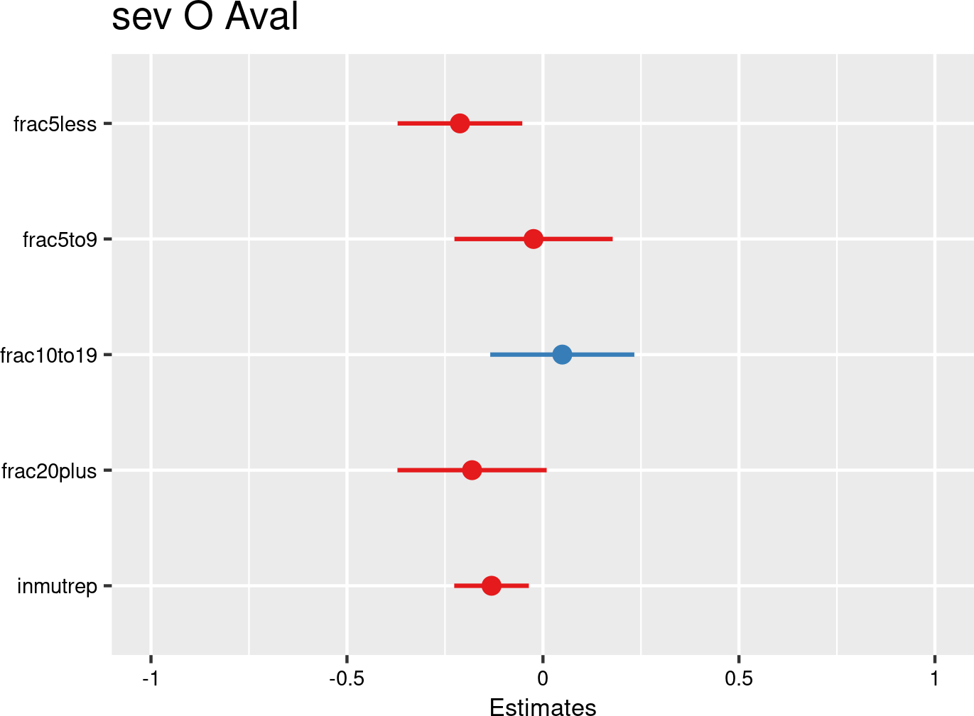

Commuting distance categories proportions were introduced as fixed effects, and companies as random effects. The model is based on data of all mutual Liantis ESPP and PS customers. The model is adjusted for representativeness of the company (fixed effect inmutrep) regarding to sector, size and Flemish province.
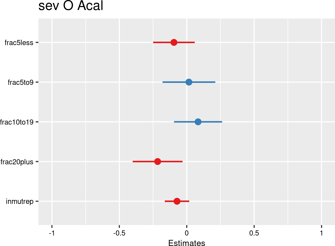

Commuting distance categories proportions were introduced as fixed effects, and companies as random effects. The model is based on data of all mutual Liantis ESPP and PS customers. The model is adjusted for representativeness of the company (fixed effect inmutrep) regarding to sector, size and Flemish province.
3.4.1.8 Use of Personal Protective Equipment (PPE)
Data Quality Alert: Use of PPE
Unfortunately and as described in Section 2.15, given the limited data, the lack of longitudinal tracking, the uneven distribution in time and other data quality issues, linking the Liantis ESPP PPE evaluation data to occupational accidents would provide a very limited and potentially misleading picture considering the small number of employees for whom data is available. As a result, no further analyses or modelling efforts were undertaken in relation to use of PPE.
3.4.1.9 Health problems: quality of hearing
Based on the parameters outlined in Section 1.3.2.9, hearing impairment qualifies as a potential determinant with objective test results available through the medical preventive consults for further investigation. The other parameters mentioned are not systematically captured in the Liantis ESPP dataset via technical test results and will not be explored further.
NSSO nor FEDRIS provide statistics concerning health problems. For this reason, a descriptives section analogous to the other univariable analyses sections does not make sense here. We will only present results of the models examining the relation between the presence of noise dips and the different outcomes of OA under investigation.
Data Quality Alert: quality of hearing
As described in Section 2.13, after initial testing, in general only employees with assigned risks related to noise exposure qualify for follow up audiometric testing during a medical prevention consult. Thus, the results will not be representative of the entire working population within (or outside) Liantis customers through the whole ten-year period of the study.
Moreover, only data from employees from mutual Liantis ESPP and PS customers can be used for modelling, further reducing the potential number of cases described by 70%.
Additionally, an important assumption was made. Because the likelihood in the first three models is assessed on a monthly basis -i.e., whether an OA occurred for a given individual in a given month- and audiometric test results are not available monthly, we interpolated the noise dip variable within individuals. Specifically, we applied an “updown” approach: once a noise dip is observed (or not), its status is assumed to persist until the next available test result for the same person. For the first available result, we assumed the condition (presence or absence of a noise dip) was already present prior to testing. Employees without any audiometric test data were excluded from the analysis.
3.4.1.9.1 Models
The following Table 3.59 summarizes the results of the models assessing the relationship between absence (0) or presence (1) of noise dips and the nine outcomes. Below the table, you can find the data on which each model is based. The results of the nine models are then presented both graphically and in a table.
| cataudio | chance to notify | chance on refusal | chance commuting | chance workplace | freq degree | chance serious | nDays TAO V/C | cost | sev degree |
|---|---|---|---|---|---|---|---|---|---|
| noise dip 0 | REF | REF | REF | REF | < | REF | REF | REF | </ns |
| noise dip 1 | > | ns | ns | > | rank def | ns | ns/> | > | rank def |
| occur | accept | occur | occur | occur | severe | severe | severe | severe | |
| empl | empl | empl | empl | comp | empl | empl | empl | comp | |
| c/w all | c/w ref | c acc | w acc | w acc | w acc | w acc | w acc | w acc |
- occur: data include all workers, chance for occurrence is calculated for the outcome
- accept: data include only workers with a notification of OA
- severe: data include only workers with an accepted OA
- c/w all: commuting and workplace accidents, including refused and accidents without decisions
- c/w ref: accepted or refused commuting and workplace accidents
- c acc: accepted commuting accidents
- w acc: accepted workplace accidents
- empl: the outcome is situated at the individual level
- comp: the outcome is situated at the company level
- nDaysTAO: number of days absenteeism related to the OA
- V/C: Validated number of days (available from FEDRIS) / Calculated number of days (based on the Liantis PS data)
Health problems: quality of hearing (ESPP audiometric test results)
- Workers experiencing noise dips show a higher likelihood of workplace occupational accidents. There was no association between the noise dip category and the likelihood of an accepted commuting occupational accident, nor with the refusal of a notified occupational accident.
- There was no observed relationship between noise dips and the likelihood of an occupational accident being categorized as serious.
- Companies with a higher proportion of workers without noise dips tend to show lower frequency and severity degrees, based on the validated number of days absent.
- The cost of an occupational accident appears to be higher for individuals experiencing noise dips, as does the number of days off calculated by Liantis PS.
- Since hearing loss worsens with age -and wage, costs, and recovery time also increase with age- the associations found are not surprising. Further research using multivariable modelling is needed to clarify whether these relationships still hold when age is included as a confounding factor.
Figure 3.81 shows that workers facing audiometric test results in which noise dips are detected, have a 7% higher chance of reporting an OA (both commuting and workplace accidents), after accounting for significant differences in company representativeness (see Section 3.2). The results suggest that hearing impairment influences the likelihood to report an OA.
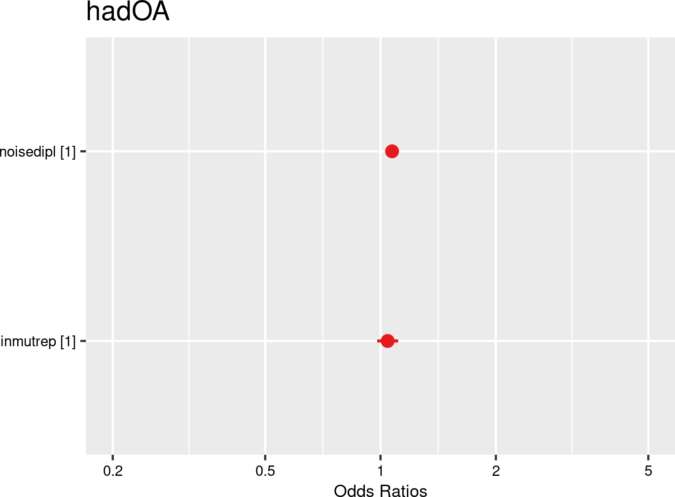

Noise dip categories were introduced as fixed effects, and companies and employees as random effects. The model is based on data from employees with and without OA from all mutual Liantis ESPP and PS customers. The model is adjusted for representativeness of the company (fixed effect inmutrep) regarding to sector, size and Flemish province.
Figure 3.82 shows that the presence of noise dips does not significantly determine whether an insurer accepts or rejects an OA claim.
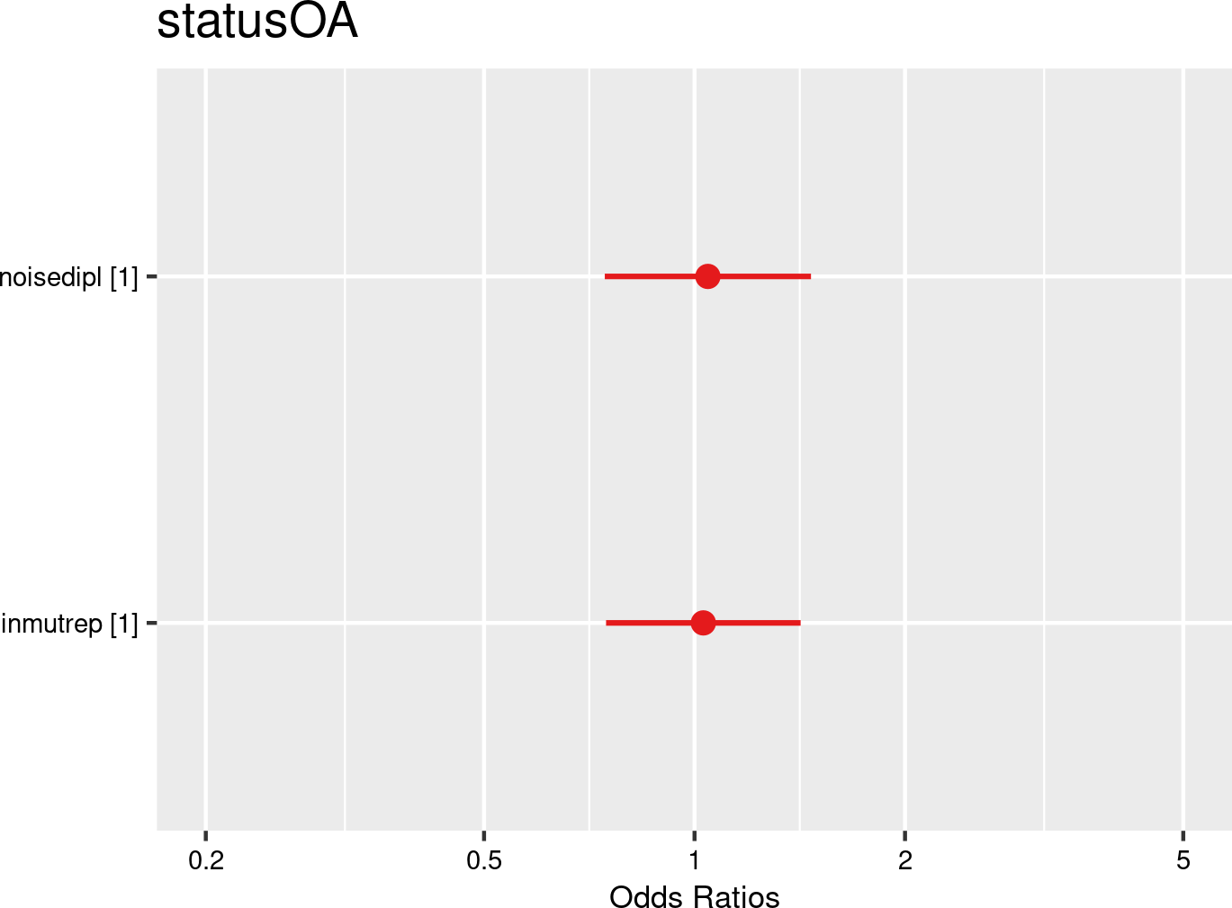

Noise dip categories were introduced as fixed effects, and companies and employees as random effects. The model is based on data from employees notifying OA from all mutual Liantis ESPP and PS customers. The model is adjusted for representativeness of the company (fixed effect inmutrep) regarding to sector, size and Flemish province.
The results presented in Figure 3.83 show no association between hearing impairment described through the presence of noise dips and the likelihood for an accepted commuting OA.
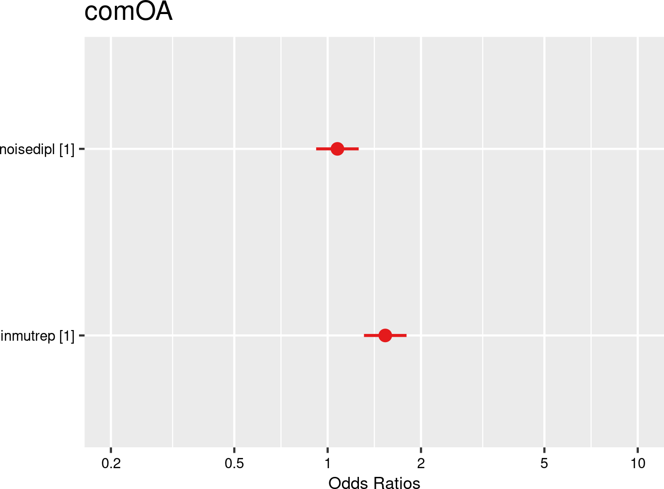

Noise dip categories were introduced as fixed effects, and companies and employees as random effects. The model is based on data from employees with and without OA from all mutual Liantis ESPP and PS customers. The model is adjusted for representativeness of the company (fixed effect inmutrep) regarding to sector, size and Flemish province.
Figure 3.84 shows that workers with noise dips have a 7% higher chance of having an accepted workplace accident compared to the reference category (without noise dips). This result indicates that hearing impairment indeed may influence the likelihood to experience an accepted workplace OA.
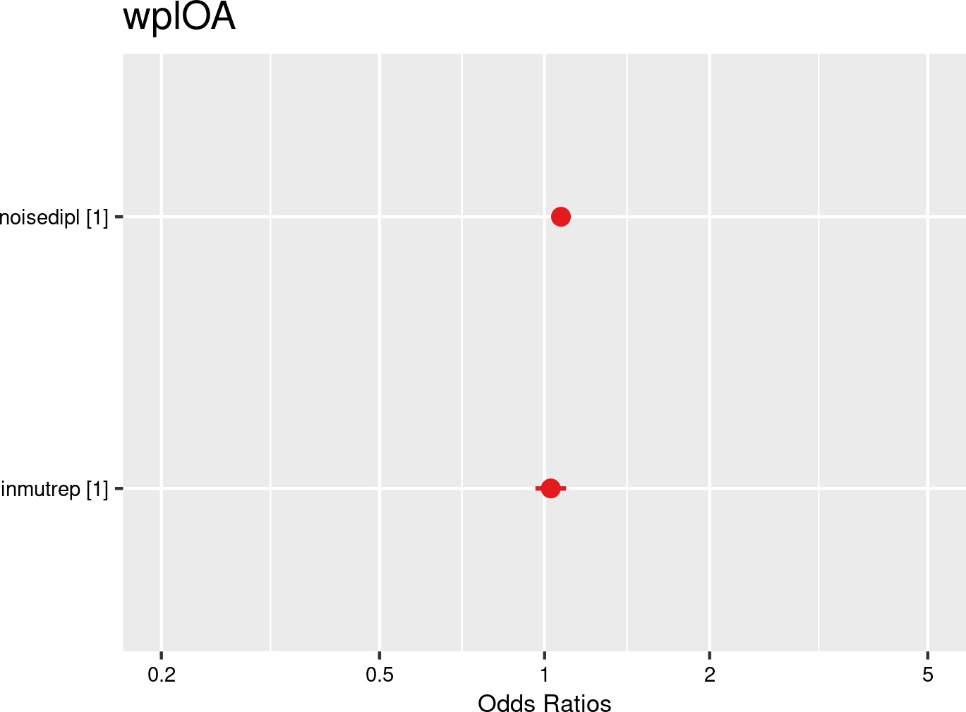

Noise dip categories were introduced as fixed effects, and companies and employees as random effects. The model is based on data from employees with and without OA from all mutual Liantis ESPP and PS customers. The model is adjusted for representativeness of the company (fixed effect inmutrep) regarding to sector, size and Flemish province.
Figure 3.85 (a) and Figure 3.85 (b) present a model estimating the frequency degree of occupational accidents at the company level, in contrast to previous models that focused on individual employee accident probabilities. These figures show that a higher proportion of workers without noise dips decreases the frequency degree of OA within a company.
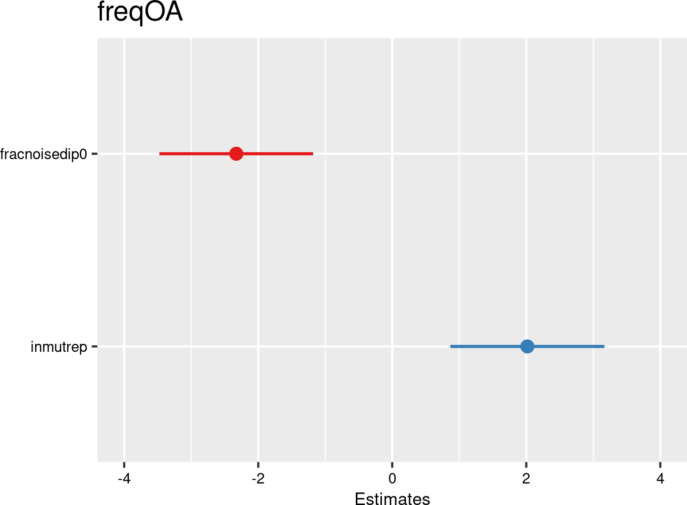

Noise dip category proportions were introduced as fixed effects, and companies as random effects. The model is based on data of all mutual Liantis ESPP and PS customers. The model is adjusted for representativeness of the company (fixed effect inmutrep) regarding to sector, size and Flemish province.
Figure 3.86 (a) and Figure 3.86 (b) present a model estimating the chance for an accepted workplace OA being classified as serious (according to the definition in the Belgian law). These figures indicate that the noise dips do not significantly determine whether an occupational workplace accident is classified as serious.
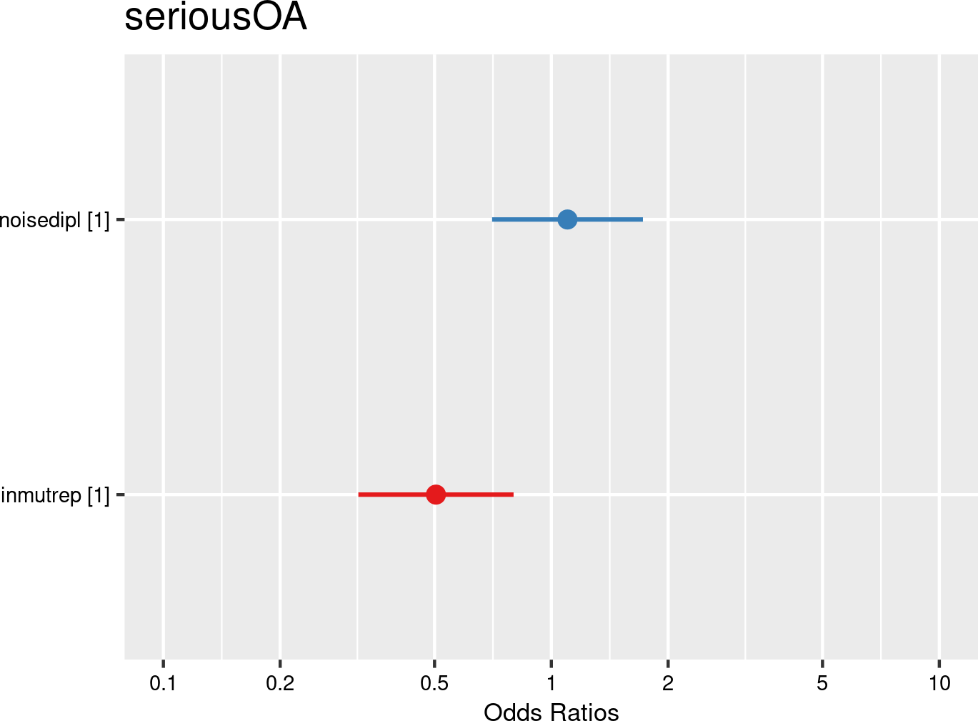

Noise dip categories were introduced as fixed effects, and companies and employees as random effects. The model is based on data of all mutual Liantis ESPP and PS customers. The model is adjusted for representativeness of the company (fixed effect inmutrep) regarding to sector, size and Flemish province.
Figure 3.87 (a) and Figure 3.87 (b) show the results of a model assessing the relation between noise dips and the number of absenteeism days. These first two figures are based on the absenteeism data provided by FEDRIS (while Figure 3.88 (a) and Figure 3.88 (b) present the same model based on the Liantis PS data). The figures show that noise dips are not important in determining the validated number of absenteeism days related to an accepted workplace OA.
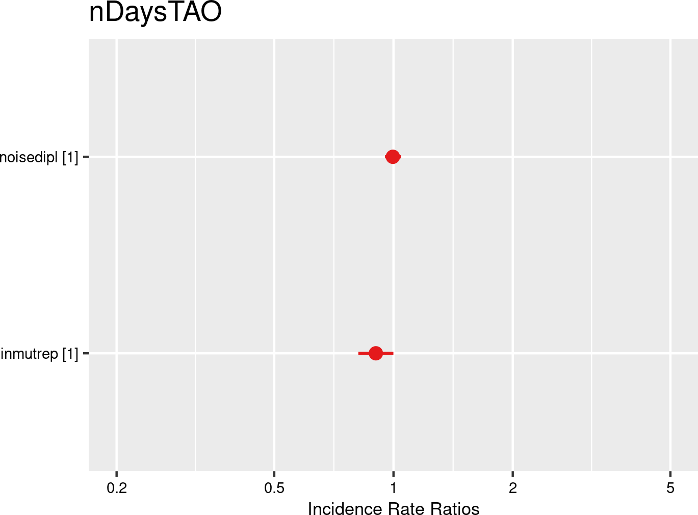

Noise dip categories were introduced as fixed effects, and companies and employees as random effects. The model is based on data of all mutual Liantis ESPP and PS customers. The model is adjusted for representativeness of the company (fixed effect inmutrep) regarding to sector, size and Flemish province.
As mentioned above, Figure 3.88 (a) and Figure 3.88 (b) are the results of the model assessing the relation between noise dip category and number of absenteeism days related to the workplace accident, based on the Liantis PS calculated data. The results are in contrast with the results of Figure 3.87 above (but the dataset used for the present model is only half in size).


Noise dip categories were introduced as fixed effects, and companies and employees as random effects. The model is based on data of all mutual Liantis ESPP and PS customers. The model is adjusted for representativeness of the company (fixed effect inmutrep) regarding to sector, size and Flemish province.
Figure 3.89 (a) and Figure 3.89 (b) show the results of the model that is assessing the relation between noise dip category and direct wage cost of an OA. It indicates that the presence of noise dips seems to be significantly related to a higher direct wage cost of an OA for an employer.
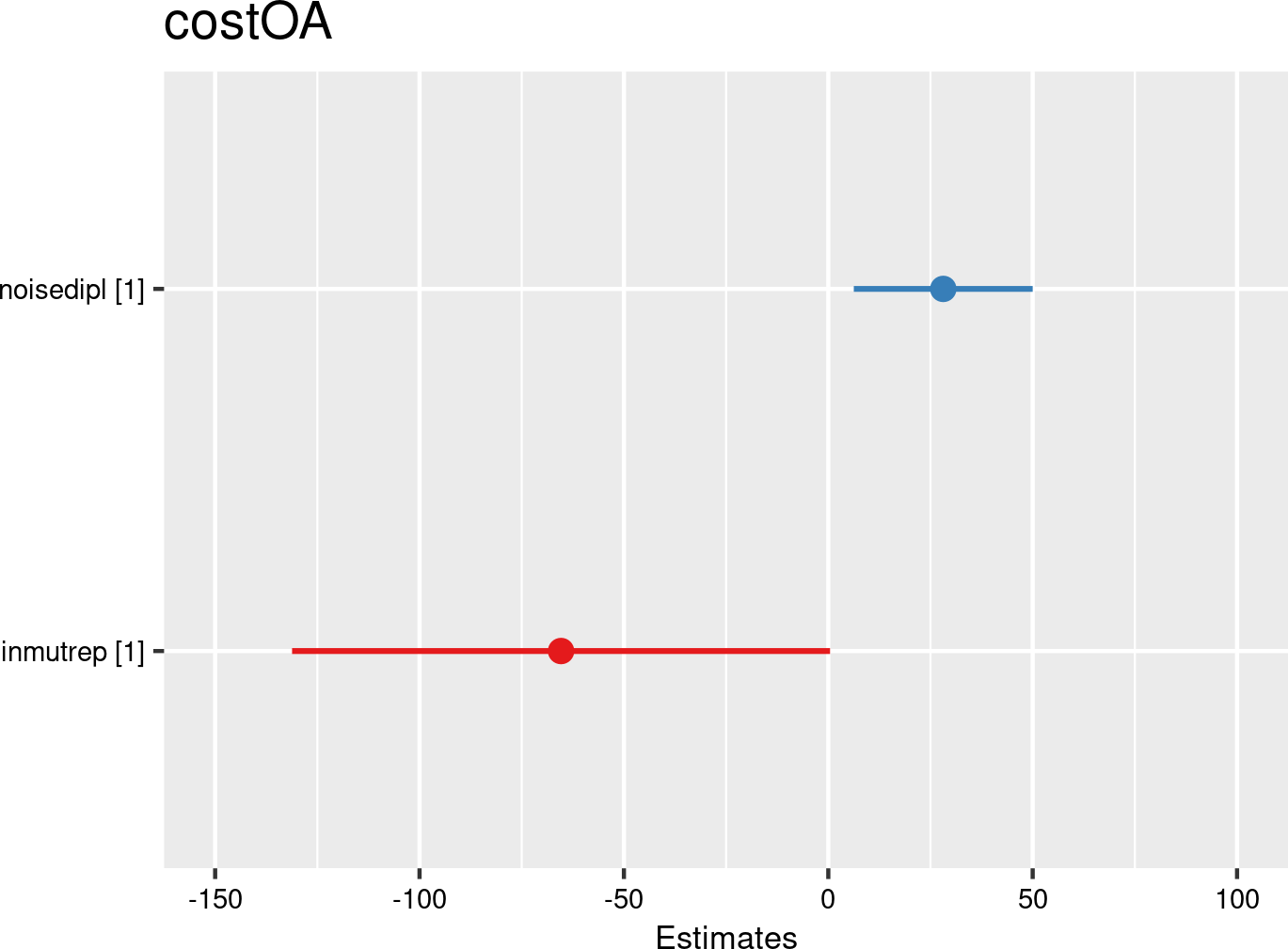

Noise dip categories were introduced as fixed effects, and companies and employees as random effects. The model is based on data of all mutual Liantis ESPP and PS customers. The model is adjusted for representativeness of the company (fixed effect inmutrep) regarding to sector, size and Flemish province.
The next 4 figures (Figure 3.90 (a) and Figure 3.90 (b), Figure 3.91 (a) and Figure 3.91 (b)) are displaying the results of a model assessing the relation between proportion of workers with (and without) noise dips and the severity degree of a company, which is again a variable at the company level. In the first model (Figure 3.90), the validated number of absenteeism days from FEDRIS was used, while the second model (Figure 3.91) was based on the numbers of days off calculated from the Liantis PS data. These figures show that a higher proportion of workers without noise dips decreases the severity degree within a company.
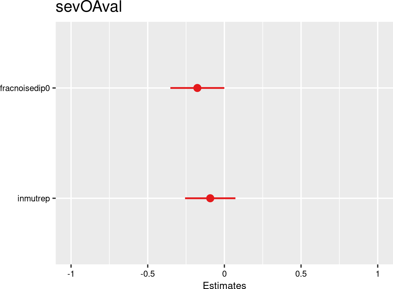

Noise dip category proportions were introduced as fixed effects, and companies as random effects. The model is based on data of all mutual Liantis ESPP and PS customers. The model is adjusted for representativeness of the company (fixed effect inmutrep) regarding to sector, size and Flemish province.
Figure 3.91 shows that a higher proportion of workers without noise dips does not significantly decreases the severity degree within a company, based on the number of calculated days from Liantis PS data. The direction of the (insignificant) effect is however in line with the conclusion from the previous model using validated FEDRIS data.
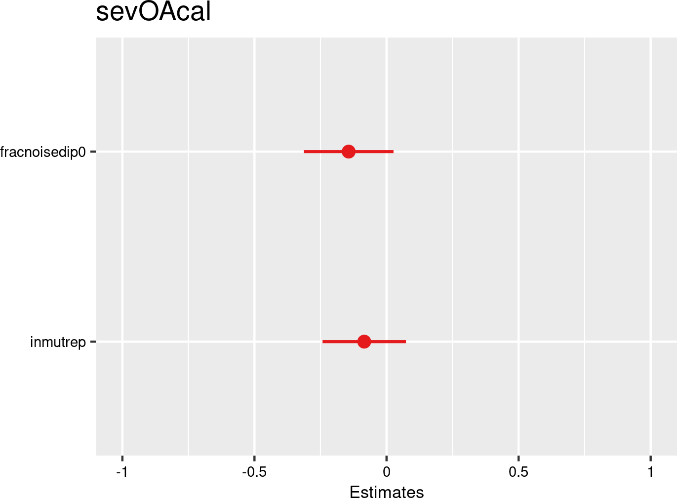

Nois dip category proportions were introduced as fixed effects, and companies as random effects. The model is based on data of all mutual Liantis ESPP and PS customers. The model is adjusted for representativeness of the company (fixed effect inmutrep) regarding to sector, size and Flemish province.
3.4.1.10 Sleeping disorders
Data Quality Alert: sleeping disorders
- Only limited data is available (from March 2022 to December 2023, see Section 2.14)
- Information comes from the General Medical Questionnaire (AMV in Dutch) (GMQ) (self-reported)
- An assumption was made (fill downup between questionnaire moments within person) to complete missing monthly data
- We only present a (preliminary) result without undertaking any further modelling efforts
Descriptives on the relation between self-reported sleep problems and notifications of occupational accidents are presented in Table 3.60. A Pearson’s Chi-squared test of independence between hadOA and SLEEP PROBLEMS suggests that the effect is statistically not significant \(\chi^2 = 6.47\), \(df = 4\), \(p = 0.167\).
| 0 days | < 1 week | 1 week - 1 month | 1 month - 3 months | > 3 months | |
|---|---|---|---|---|---|
| 0 | 487157 | 116954 | 87634 | 43796 | 93339 |
| 1 | 2394 | 567 | 471 | 219 | 503 |
| 0 days | < 1 week | 1 week - 1 month | 1 month - 3 months | > 3 months | |
|---|---|---|---|---|---|
| 0 | 99.51 | 99.52 | 99.47 | 99.5 | 99.46 |
| 1 | 0.49 | 0.48 | 0.53 | 0.5 | 0.54 |
3.4.1.11 Substance abuse
Data Quality Alert: substance abuse (alcohol)
- Only limited data is available (from March 2022 to December 2023, see Section 2.14)
- Information comes from the GMQ (self-reported)
- An assumption was made (fill downup between questionnaire moments within person) to complete missing monthly data
- We only present a (preliminary) result without undertaking any further modelling efforts
Descriptives on the relation between self-reported alcohol consumption and notifications of occupational accidents are presented in Table 3.61. A Pearson’s Chi-squared test of independence between hadOA and ALCOHOL CONSUMPTION suggests that the effect is statistically not significant \(\chi^2 = 6.58\), \(df = 5\), \(p = 0.254\).
| No | <= 5 | 6 - 10 | 11 - 20 | > 20 | I do not wish to answer | |
|---|---|---|---|---|---|---|
| 0 | 16837 | 20333 | 5846 | 1452 | 317 | 1060 |
| 1 | 98 | 95 | 22 | 10 | 2 | 3 |
| No | <= 5 | 6 - 10 | 11 - 20 | > 20 | I do not wish to answer | |
|---|---|---|---|---|---|---|
| 0 | 99.42 | 99.53 | 99.63 | 99.32 | 99.37 | 99.72 |
| 1 | 0.58 | 0.47 | 0.37 | 0.68 | 0.63 | 0.28 |
Data Quality Alert: substance abuse (drugs)
- Only limited data is available (from March 2022 to December 2023, see Section 2.14)
- Information comes from the GMQ (self-reported)
- An assumption was made (fill downup between questionnaire moments within person) to complete missing monthly data
- We only present a (preliminary) result without undertaking any further modelling efforts
Descriptives on the relation between self-reported drug use and notifications of occupational accidents are presented in Table 3.62. A Pearson’s Chi-squared test of independence between hadOA and DRUG USE suggests that the effect is statistically not significant \(\chi^2 = 4.77\), \(df = 3\), \(p = 0.189\).
| No | Occasionally | Every day | I do not wish to answer | |
|---|---|---|---|---|
| 0 | 44367 | 954 | 147 | 377 |
| 1 | 222 | 8 | 0 | 0 |
| No | Occasionally | Every day | I do not wish to answer | |
|---|---|---|---|---|
| 0 | 99.5 | 99.17 | 100 | 100 |
| 1 | 0.5 | 0.83 | 0 | 0 |
Data Quality Alert: medication use
- Only limited data is available (from March 2022 to December 2023, see Section 2.14)
- Information comes from the GMQ (self-reported)
- An assumption was made (fill downup between questionnaire moments within person) to complete missing monthly data
- We only present a (preliminary) result without undertaking any further modelling efforts
Descriptives on the relation between self-reported medication use and notifications of occupational accidents are presented in Table 3.63. A Pearson’s Chi-squared test of independence between hadOA and MEDICATION suggests that the effect is statistically not significant \(\chi^2 = 3.52\), \(df = 3\), \(p = 0.318\).
| Nee | Af en toe | Dagelijks | Wil niet antwoorden | |
|---|---|---|---|---|
| 0 | 39147 | 3966 | 2440 | 292 |
| 1 | 191 | 26 | 13 | 0 |
| Nee | Af en toe | Dagelijks | Wil niet antwoorden | |
|---|---|---|---|---|
| 0 | 99.51 | 99.35 | 99.47 | 100 |
| 1 | 0.49 | 0.65 | 0.53 | 0 |
3.4.1.12 Personality
Data Quality Alert: personality
Within Liantis, no systematically maintained variables related to personality traits are currently available that would allow for investigation of a potential association with occupational accidents. Similarly, the FEDRIS notification data does not include any variables related to personality traits. As a result, no further analyses or modelling efforts were undertaken in relation to personality characteristics.
3.4.1.13 Number of years of schooling
Data Quality Alert: number of years of schooling
Within Liantis, no systematically maintained variables related to the number of years of schooling are currently available that would allow for investigation of a potential association with occupational accidents. Similarly, the FEDRIS notification data does not include any variables related to number of years of schooling. As a result, no further analyses or modelling efforts were undertaken in relation to number of years of schooling.
3.4.2 Job related factors
3.4.2.1 Occupation and workforce segment
Data Quality Alert: Occupation and workforce segment
In the data quality report section, we examined three variables on their suitability as a proxy for occupation and workforce segment: catnsso, catprof, and catisco (see Section 2.7.2.3, Section 2.7.2.5 and Section 2.7.2.6). Although there are also some issues with the data from catnsso variable in the notifications, it seems a better choice than catprof and certainly catisco (since the tag is almost always missing for this last one, a mapping the the International Standard Classification of Occupations (ISCO) system will not be possible). With catnsso we see less NA or “Onbekend” values and a slightly better mapping to blue and white collar workers. For this reason, we will only examine the catnsso variable in further analyses and modelling.
3.4.2.1.1 Descriptives
The statute or employment type generally refers to the distinction between white and blue collars. The NSSO does provide data about the statute in three categories in their broadest categorisation: white collar workers, blue collar workers and civil servants). FEDRIS statistical reports and notifications provide information about the statute, although they include a lot more categories. Since Liantis PS data also contains the indication of a white collar, blue collar or other worker, this variable could be categorised in the same categories that are used in the NSSO reports. On the other hand, the FEDRIS statistical reports and the FEDRIS notification data had to be recategorized into larger categories. Hereafter, the fit between the derived statute category of an employee experiencing an OA can be compared with the corresponding statute category classification in the notification of the accident.
From Figure 3.92 we learn that the nature of the statute categories of Liantis PS data and FEDRIS data are quite comparable. This suggests that the statute categories derived from Liantis PS data might align well with those in FEDRIS data, making them suitable for further analysis. The accuracy is >98%.
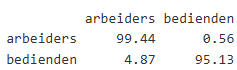
In the next 6 tables, an overview of all (accepted) OAs (Table 3.64 and Table 3.65), the commuting OAs (Table 3.66 and Table 3.67) and the workplace OAs (Table 3.68 and Table 3.69) are given. In the first table ((Table 3.64, Table 3.66 and Table 3.68), the absolute numbers are provided stratified per statute category, next to the total number of employees, as available in the Liantis database. In the second table (Table 3.65, Table 3.67 and Table 3.69), the relative numbers of the OAs per statute category are provided as percentages.
From tables Table 3.65, Table 3.67, and Table 3.69, several important findings emerge. We observe a difference between NSSO and Liantis data: NSSO has more white-collar workers, while Liantis has more blue-collar workers. However, the proportion of accidents is consistently higher among blue-collar workers than expected based on the NSSO or Liantis population distribution. Conversely, the proportion of accidents among white-collar workers is lower than expected. This suggests that the risk of accidents is higher for blue-collar workers, which aligns with expectations. Additionally, the proportion of accidents among civil servants is lower than expected based on the NSSO or Liantis population distribution. This suggests that blue-collar workers are at greater risk for OAs.
all accepted occupational accidents
| name | rszall | rszpriv | liaall | fedrisall | totalnot | totalnotmut | totalnotrepmutflan |
|---|---|---|---|---|---|---|---|
| andere | NA | NA | 1611584 | 23380 | 21293 | 3215 | 2047 |
| arbeiders | 52888328 | 48618314 | 9189273 | 849555 | 121324 | 43085 | 15954 |
| bedienden | 79911613 | 65816512 | 7242032 | 480442 | 52602 | 14935 | 8029 |
| name | percrszall | percrszpriv | percliaall | percfedrisall | perctotalnot | perctotalnotmut | perctotalnotrepmutflan |
|---|---|---|---|---|---|---|---|
| andere | NA | NA | NA | NA | NA | NA | NA |
| arbeiders | 39.83 | 42.49 | 55.9 | 63.9 | 69.8 | 74.3 | 66.5 |
| bedienden | 60.17 | 57.51 | 44.1 | 36.1 | 30.2 | 25.7 | 33.5 |
commuting accepted occupational accidents
| name | rszall | rszpriv | liaall | fedrisall | totalnot | totalnotmut | totalnotrepmutflan |
|---|---|---|---|---|---|---|---|
| andere | NA | NA | 1611584 | 4083 | 3663 | 407 | 240 |
| arbeiders | 52888328 | 48618314 | 9189273 | 95916 | 11783 | 4436 | 1951 |
| bedienden | 79911613 | 65816512 | 7242032 | 126311 | 12941 | 3756 | 1921 |
| name | percrszall | percrszpriv | percliaall | percfedrisall | perctotalnot | perctotalnotmut | perctotalnotrepmutflan |
|---|---|---|---|---|---|---|---|
| andere | NA | NA | NA | NA | NA | NA | NA |
| arbeiders | 39.83 | 42.49 | 55.9 | 43.2 | 47.7 | 54.2 | 50.4 |
| bedienden | 60.17 | 57.51 | 44.1 | 56.8 | 52.3 | 45.8 | 49.6 |
workplace accepted occupational accidents
| name | rszall | rszpriv | liaall | fedrisall | totalnot | totalnotmut | totalnotrepmutflan |
|---|---|---|---|---|---|---|---|
| andere | NA | NA | 1611584 | 19297 | 17630 | 2808 | 1807 |
| arbeiders | 52888328 | 48618314 | 9189273 | 753639 | 109541 | 38649 | 14003 |
| bedienden | 79911613 | 65816512 | 7242032 | 354131 | 39661 | 11179 | 6108 |
| name | percrszall | percrszpriv | percliaall | percfedrisall | perctotalnot | perctotalnotmut | perctotalnotrepmutflan |
|---|---|---|---|---|---|---|---|
| andere | NA | NA | NA | NA | NA | NA | NA |
| arbeiders | 39.83 | 42.49 | 55.9 | 68 | 73.4 | 77.6 | 69.6 |
| bedienden | 60.17 | 57.51 | 44.1 | 32 | 26.6 | 22.4 | 30.4 |
3.4.2.1.2 Models
The following Table 3.70 summarizes the results of the models assessing the relationship between contract and the several outcomes related to OAs. Below the table, details are provided about the data used for the analyses. The results of the nine models are then presented both in a table and graphically.
| catnsso | chance to notify | chance on refusal | chance commuting | chance workplace | freq degree | chance serious | nDays TAO V/C | cost | sev degree V/C |
|---|---|---|---|---|---|---|---|---|---|
| blue collars | REF | REF | REF | REF | > | REF | REF | REF | >/> |
| white collars | < | ns | > | < | ns | < | </< | < | </< |
| occur | accept | occur | occur | occur | severe | severe | severe | severe | |
| empl | empl | empl | empl | comp | empl | empl | empl | comp | |
| c/w all | c/w ref | c acc | w acc | w acc | w acc | w acc | w acc | w acc |
- occur: data include all workers, chance for occurrence is calculated for the outcome
- accept: data include only workers with a notification of OA
- severe: data include only workers with an accepted OA
- c/w all: commuting and workplace accidents, including refused and accidents without decisions
- c/w ref: accepted or refused commuting and workplace accidents
- c acc: accepted commuting accidents
- w acc: accepted workplace accidents
- empl: the outcome is situated at the individual level
- comp: the outcome is situated at the company level
- nDaysTAO: number of days absenteeism related to the OA
- V/C: Validated number of days (available from FEDRIS) / Calculated number of days (based on the Liantis PS data)
Occupation and workforce segment and occupational accidents
- Blue collars have a higher chance to report an occupational accident (and have a higher chance for an accepted workplace occupational accident)
- Blue collars have a higher chance for an occupational accident being serious.
- Blue collars have more absenteeism days related to an occupational accident, including more wage related costs for the employer.
- A higher proportion of blue collars increases the frequency and severity degree within a company.
According to Figure 3.93 (a) and Figure 3.93 (b), white collars are 63% less likely to report OAs (both commuting and workplace accidents) compared to blue collar workers, even after accounting for significant differences in company representativeness. This is in line with expectations and former research (Abatemarco et al., 1995; Hägg et al., 2015).
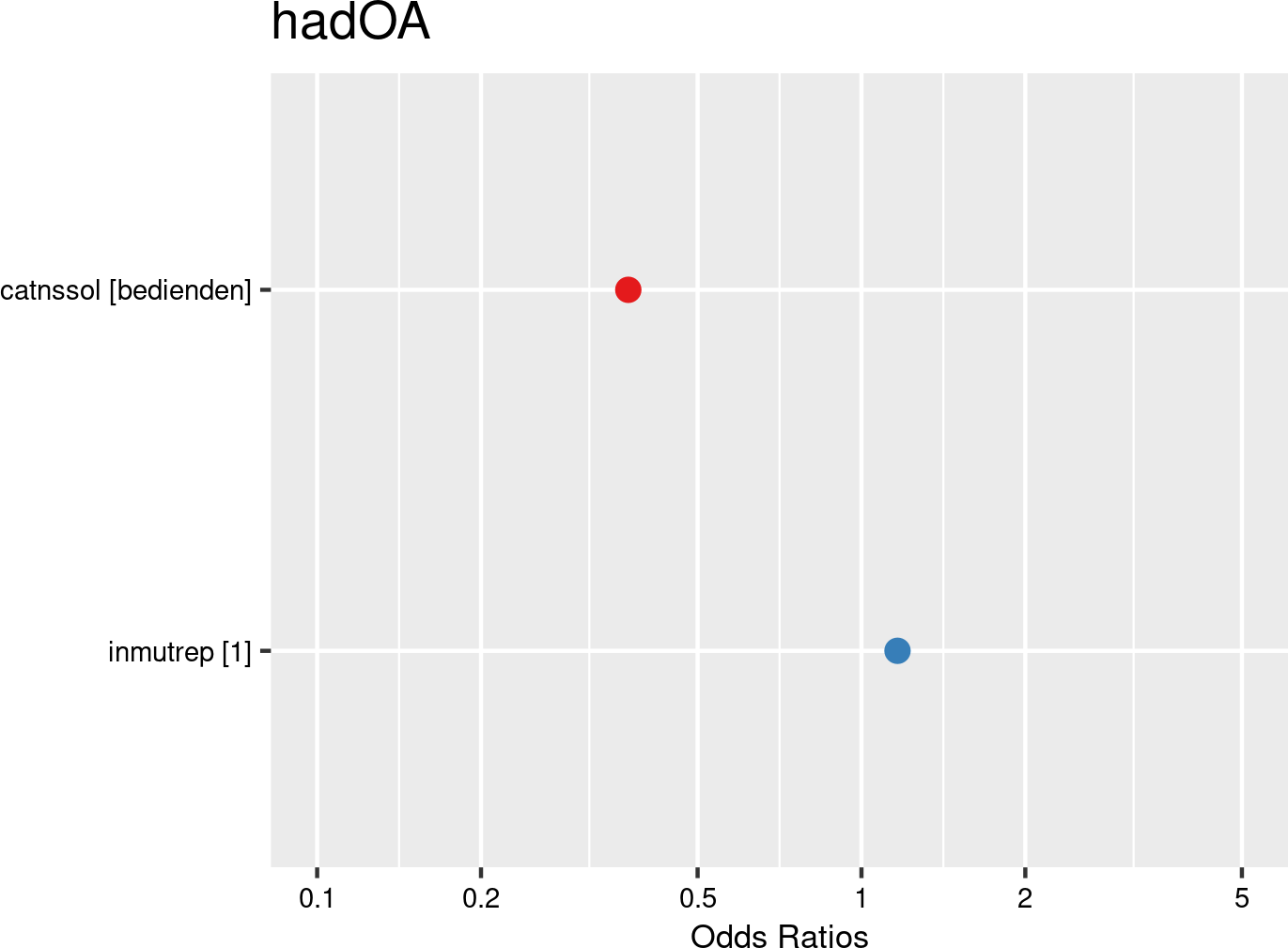

Statute type categories were introduced as fixed effects, and companies and employees as random effects. The model is based on data from employees with and without OAs from all mutual Liantis ESPP and PS customers. The model is adjusted for representativeness of the company (fixed effect inmutrep) regarding to sector, size and Flemish province.
According to Figure 3.94 (a) and Figure 3.94 (b), the statute does not significantly determine the likelihood of a reported OA being rejected by the insurer.
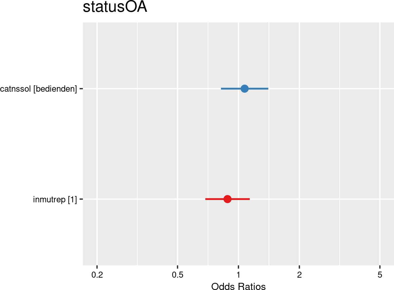

Statute categories were introduced as fixed effects, and companies and employees as random effects. The model is based on data from employees notifying OAs from all mutual Liantis ESPP and PS customers. The model is adjusted for representativeness of the company (fixed effect inmutrep) regarding to sector, size and Flemish province.
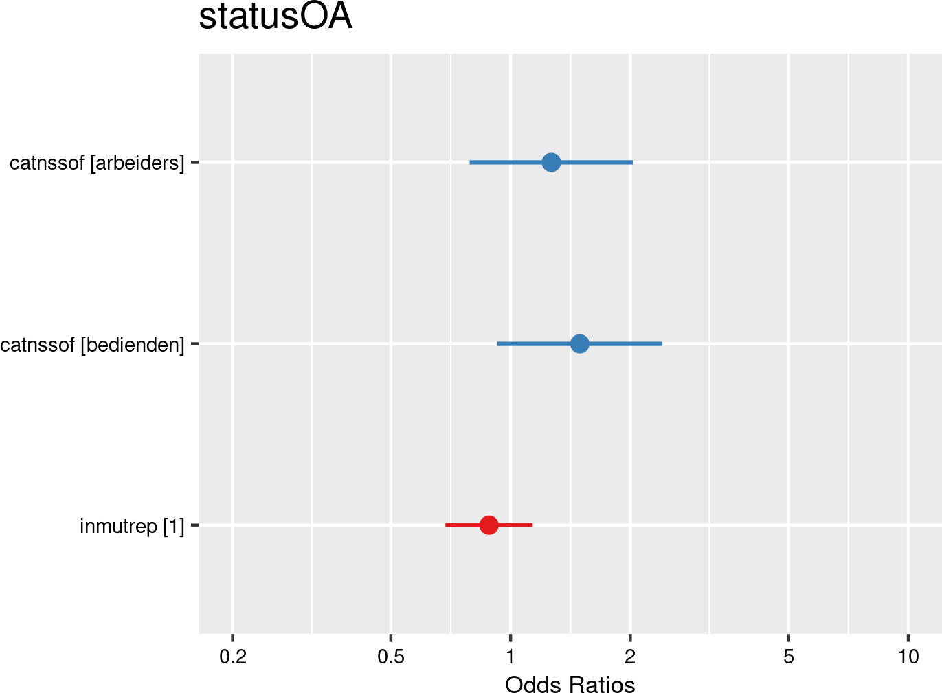

Statute categories were introduced as fixed effects, and companies and employees as random effects. The model is based on data of all employees. The model is adjusted for representativeness of the company (fixed effect inmutrep) regarding to sector, size and Flemish province.
According to Figure 3.96 (a) and Figure 3.96 (b), white-collar workers show a 21% higher chance to experience an accepted commuting accident.
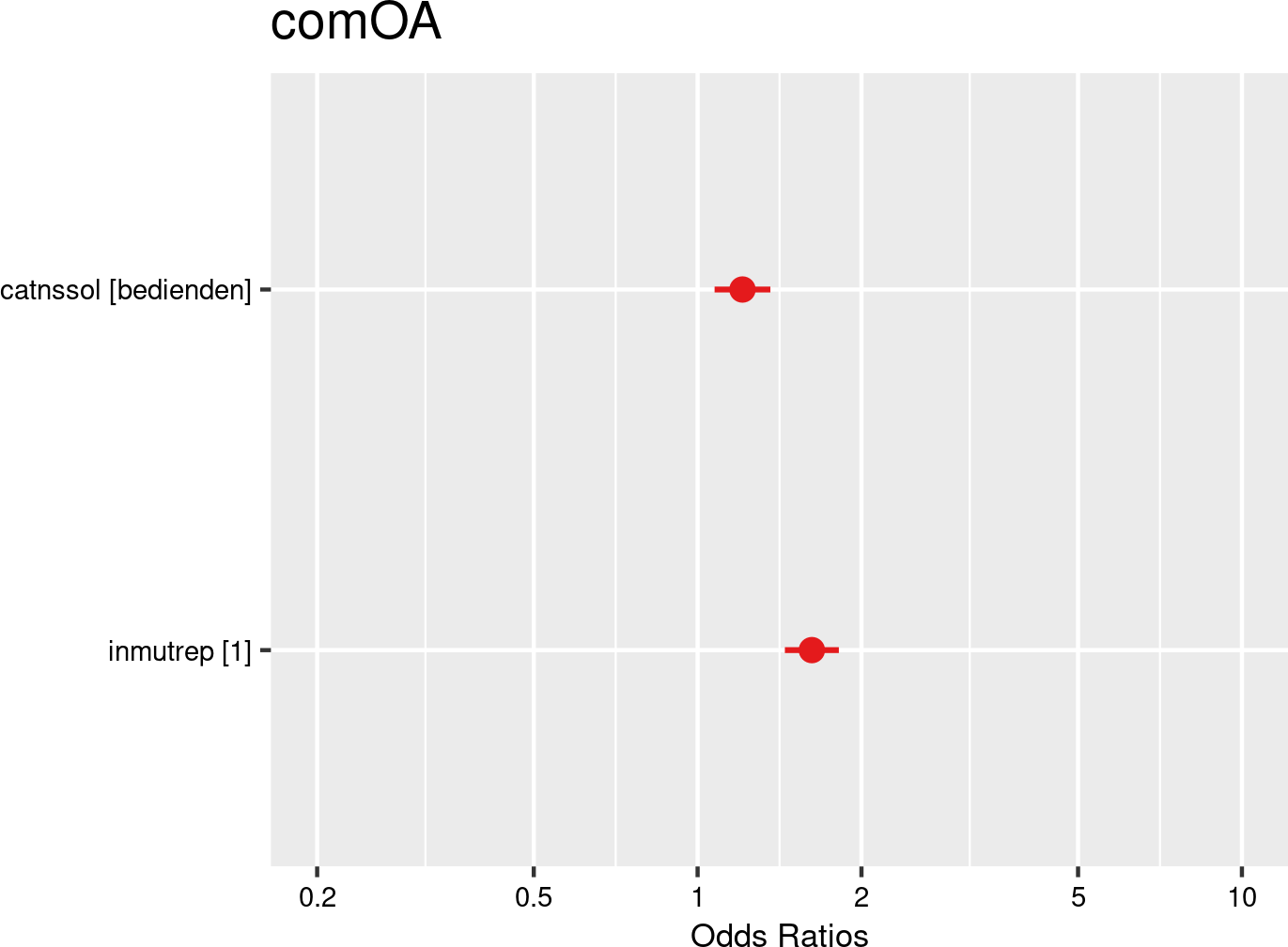

Statute categories were introduced as fixed effects, and companies and employees as random effects. The model is based on data from employees with and without OAs from all mutual Liantis ESPP and PS customers. The model is adjusted for representativeness of the company (fixed effect inmutrep) regarding to sector, size and Flemish province.
Figure 3.97 (a) and Figure 3.97 (b) show the estimates for the relation between statute categories and an accepted workplace OA. White collars have 69% less chance to experience accepted workplace accidents compared to blue collars. This is in line with expectations and former research ((Abatemarco et al., 1995; Hägg et al., 2015).
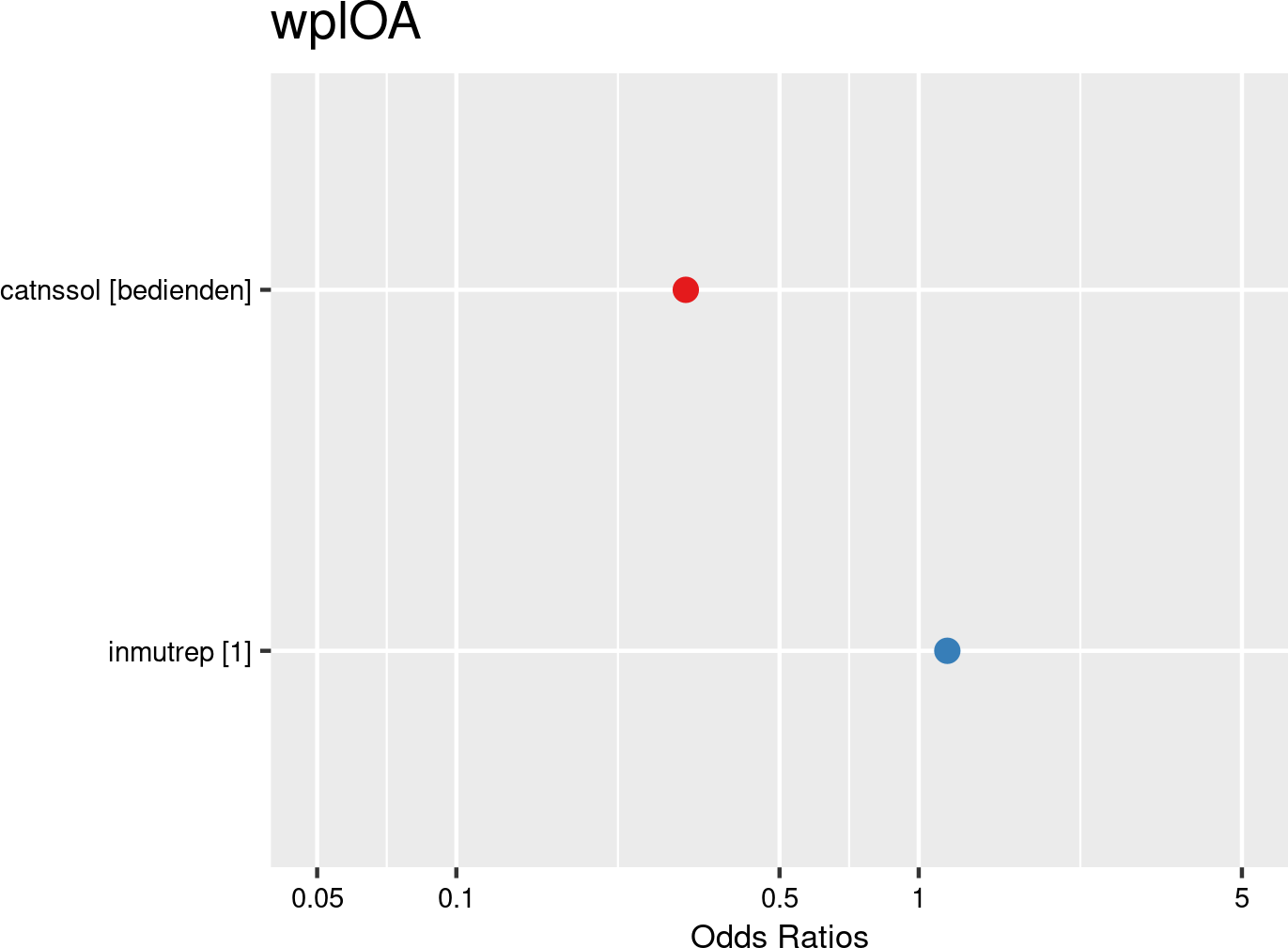

Statute type categories were introduced as fixed effects, and companies and employees as random effects. The model is based on data from employees with and without OAs from all mutual Liantis ESPP and PS customers. The model is adjusted for representativeness of the company (fixed effect inmutrep) regarding to sector, size and Flemish province.
Figure 3.98 (a) and Figure 3.98 (b) present a model estimating the frequency degree of OAs at the company level, contrasting with previous models that focused on individual employee accident probabilities. These figures show that a higher proportion of blue-collar workers significantly increases the frequency degree of OAs within a company. This aligns with expectations, as blue-collar workers are generally more exposed to safety risks.
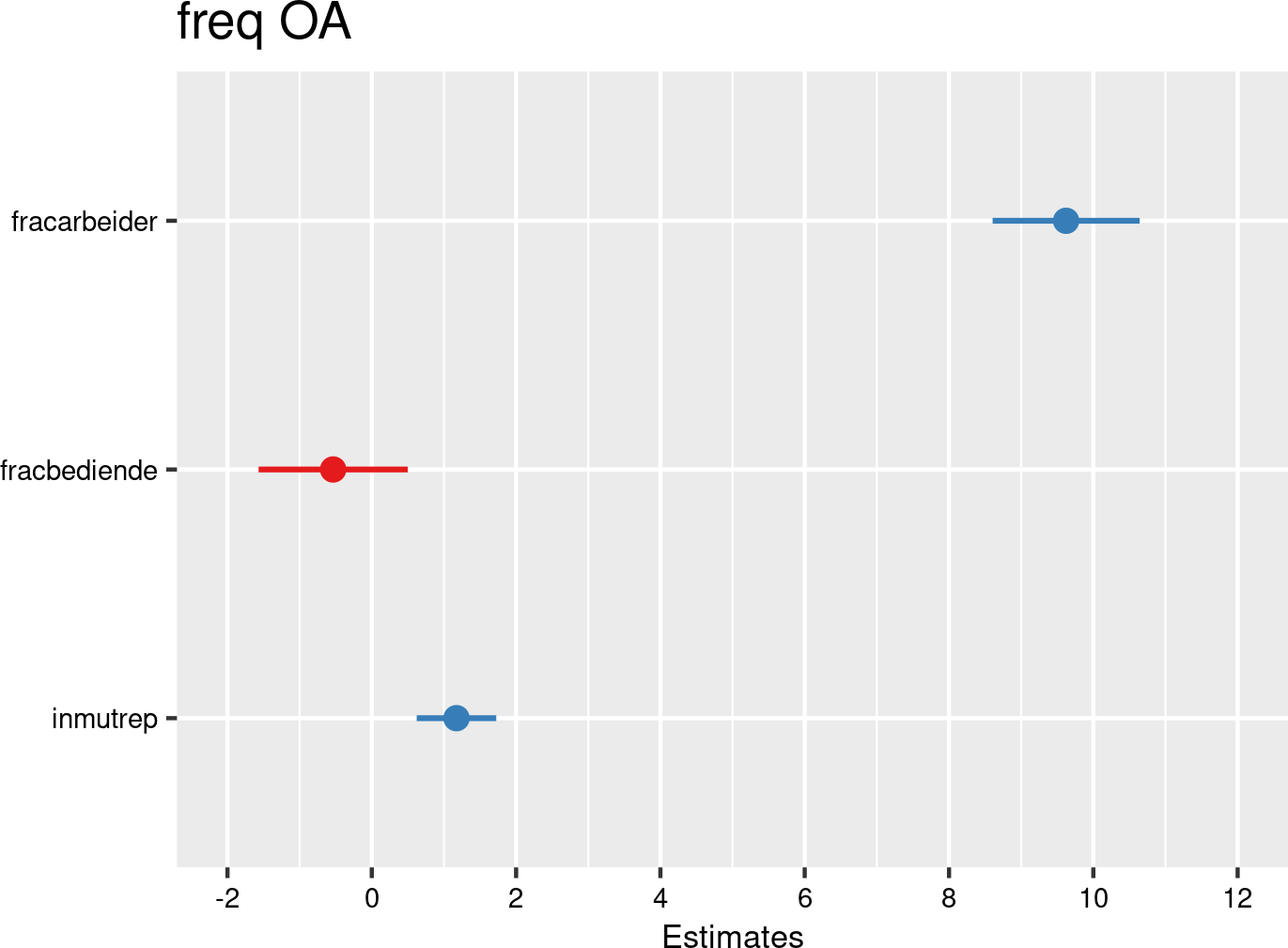

Statute categories proportions were introduced as fixed effects, and companies as random effects. The model is based on data of all mutual Liantis ESPP and PS customers. The model is adjusted for representativeness of the company (fixed effect inmutrep) regarding to sector, size and Flemish province.
Figure 3.99 (a) and Figure 3.99 (b) present a model estimating the likelihood of an accepted accident being classified as serious according to Belgian law. These figures indicate that OAs among white-collar workers are significantly less likely to be classified as serious compared to those among blue-collar workers. This aligns with expectations: as mentioned above, blue collars are are generally more exposed to safety risks.
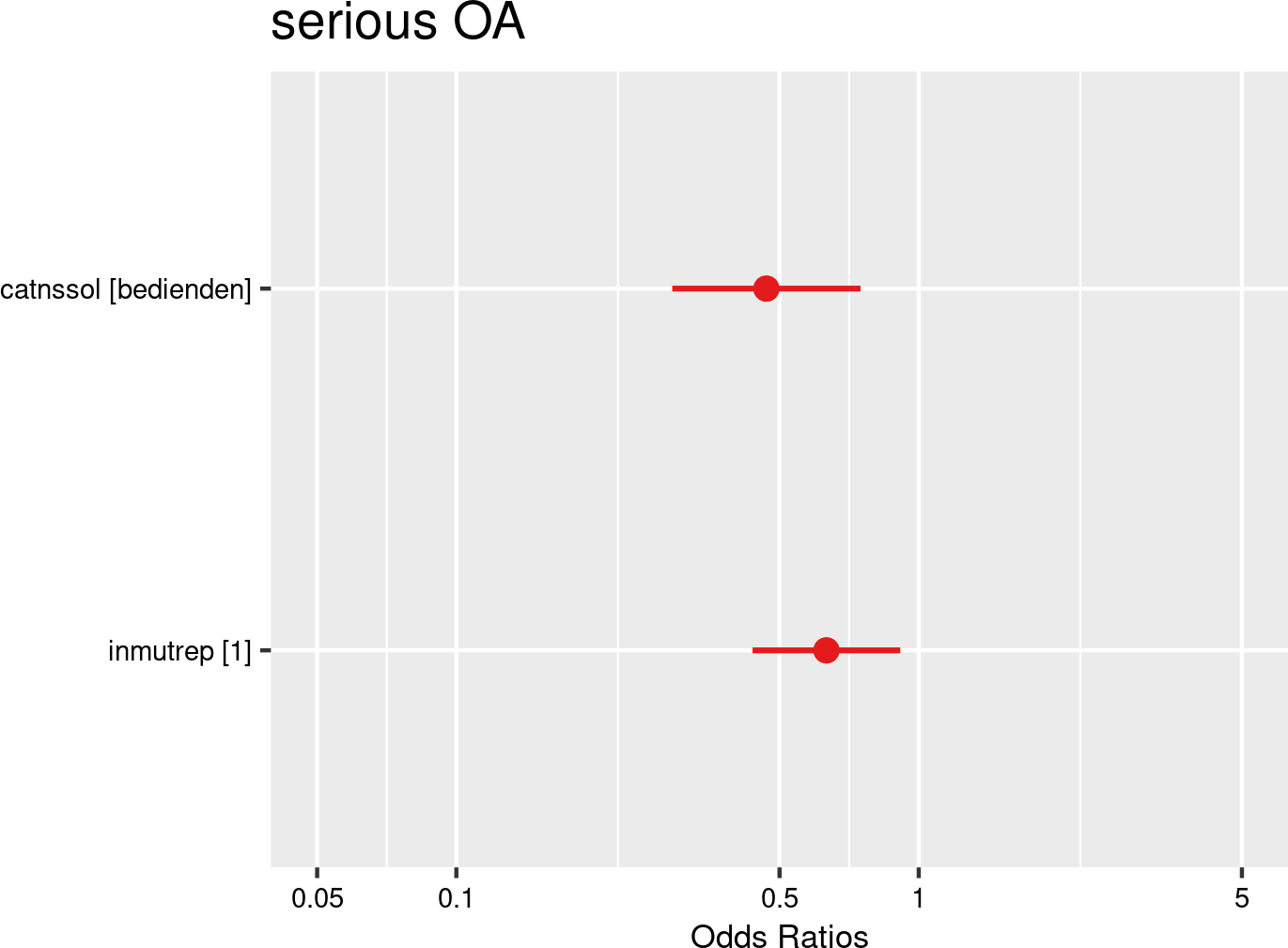

Statute categories were introduced as fixed effects, and companies and employees as random effects. The model is based on data of all mutual Liantis ESPP and PS customers. The model is adjusted for representativeness of the company (fixed effect inmutrep) regarding to sector, size and Flemish province.
Figure 3.100 (a) and Figure 3.100 (b) show the results of a model assessing the relationship between statute and the number of absenteeism days. These figures are based on absenteeism data from FEDRIS, while Figure 3.101 (a) and Figure 3.101 (b) present the same model using data from Liantis PS. The figures indicate that statute is a significant factor in determining the validated number of absenteeism days due to OAs. The number of accepted days off decreases significantly for white collars (31% less days for white collars in comparison with blue collars).
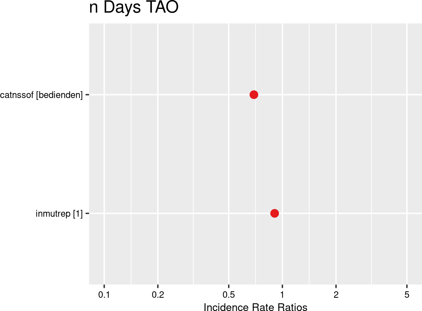

Statute categories were introduced as fixed effects, and companies and employees as random effects. The model is based on data of all mutual Liantis ESPP and PS customers. The model is adjusted for representativeness of the company (fixed effect inmutrep) regarding to sector, size and Flemish province.
As mentioned above, Figure 3.101 (a) and Figure 3.101 (b) are the results of the model assessing the relation between contract type and number of absenteeism days related to the workplace accident, based on the Liantis PS data. The findings aligns with those of the model based on the FEDRIS absenteeism data, showing white collars having less absenteeism days related to OAs then blue collars. However, the estimate is much smaller (only 6% less days for white collars, in comparison with 31% in the first model). This may be due to the smaller sample size of the Liantis PS data. In any case, these findings are consistent with expectations and the results of previous models.
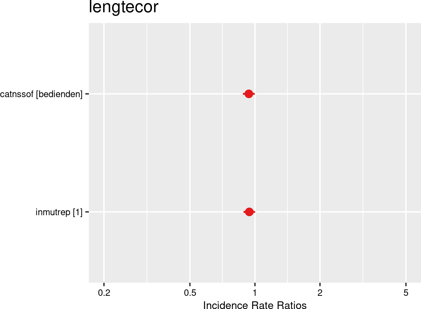

Statute type categories were introduced as fixed effects, and companies and employees as random effects. The model is based on data of all mutual Liantis ESPP and PS customers. The model is adjusted for representativeness of the company (fixed effect inmutrep) regarding to sector, size and Flemish province.
Figure 3.102 (a) and Figure 3.102 (b) show the results of a model evaluating the relationship between statute and the direct wage cost of an OA. The findings indicate that the statute significantly impacts the direct wage cost for employers: white collars incur lower costs compared to blue collars.
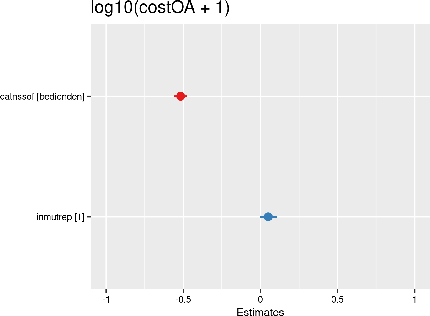

Statute categories were introduced as fixed effects, and companies and employees as random effects. The model is based on data of all mutual Liantis ESPP and PS customers. The model is adjusted for representativeness of the company (fixed effect inmutrep) regarding to sector, size and Flemish province.
The next 4 figures (Figure 3.103 (a) and Figure 3.103 (b), Figure 3.104 (a) and Figure 3.104 (b)) are displaying the results of a model assessing the relation between proportion of workers within a statute category and the severity degree of a company, which is again a variable at the company level. In the first model (Figure 3.103 (a) and Figure 3.103 (b)), validated number of absenteeism days from FEDRIS were used, while the second model Figure 3.104 (a) and Figure 3.104 (b)) was based on the numbers of days off in the Liantis PS data. The results of both models indicate that a higher proportion of blue collars significantly increases the severity level within a company. On the other hand, a higher proportion of white collars significantly decreases the severity level within a company.
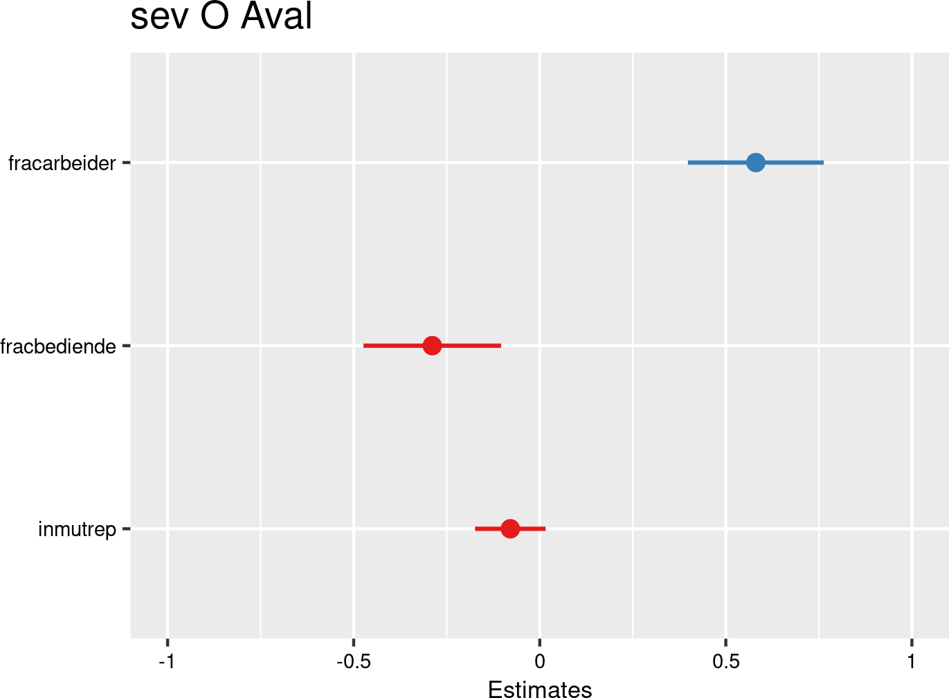

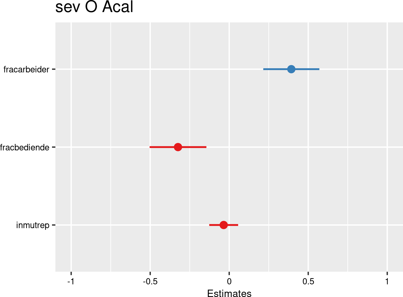

3.4.2.2 Contract type (permanent/indefinite/unlimited versus temporary/definite/limited) (precarious employment)
3.4.2.2.1 Descriptives
When we refer to contract type, we mean the duration of the contract. Generally, the distinction is made between permanent (indefinite or unlimited) and temporary (definite, fixed-term, or limited) contracts. The NSSO does not provide data on contract type. FEDRIS statistical reports and notifications include information about contract type in three categories: limited, unlimited, and unknown. In the Liantis PS dataset available for this project, contract type is not explicitly mentioned in terms of duration. Therefore, we categorize workers who have more than one contract per month as having a temporary (or limited duration) contract, while others are considered to have a permanent (or unlimited) contract.
Data Quality Alert: Contract type (permanent/indefinite/unlimited versus temporary/definite/limited) (precarious employment)
In the Liantis PS dataset available for this project, contract type is not explicitly mentioned in terms of duration. Therefore, we categorize workers who have more than one contract per month as having a temporary (or limited duration) contract, while others are considered to have a permanent (or unlimited) contract.
This is an assumption that may not always hold true, results have to be interpreted with caution.
In the next 6 tables, an overview of all (accepted) OAs (Table 3.71 and Table 3.72), the commuting OAs (Table 3.73 and Table 3.74) and the workplace OAs (Table 3.75 and Table 3.76) are given.
In the first table ((Table 3.71, Table 3.73 and Table 3.75), the absolute numbers are provided stratified per contract type category, next to the total number of employees, as available in the Liantis database.
In the second table (Table 3.72, Table 3.74 and Table 3.76), the relative numbers of the OAs per contract type category are provided as percentages.
From the table Table 3.72, it can be noticed that workers with an unlimited contract account for 79% of the employees within Liantis customers, while they account for about 88% of the employees within the notifications.
all accepted occupational accidents
| name | rszall | rszpriv | liaall | fedrisall | totalnot | totalnotmut | totalnotrepmutflan |
|---|---|---|---|---|---|---|---|
| unlimited | NA | NA | 14333967 | NA | 149146 | 42873 | 19094 |
| limited | NA | NA | 3721899 | NA | 17857 | 5881 | 2676 |
| unknown | NA | NA | NA | NA | 28216 | 12481 | 4260 |
| name | percrszall | percrszpriv | percliaall | percfedrisall | perctotalnot | perctotalnotmut | perctotalnotrepmutflan |
|---|---|---|---|---|---|---|---|
| unlimited | NA | NA | 79.4 | NA | 89.3 | 87.9 | 87.7 |
| limited | NA | NA | 20.6 | NA | 10.7 | 12.1 | 12.3 |
| unknown | NA | NA | NA | NA | NA | NA | NA |
commuting accepted occupational accidents
| name | rszall | rszpriv | liaall | fedrisall | totalnot | totalnotmut | totalnotrepmutflan |
|---|---|---|---|---|---|---|---|
| unlimited | NA | NA | 14333967 | NA | 22070 | 5996 | 3015 |
| limited | NA | NA | 3721899 | NA | 2876 | 1056 | 515 |
| unknown | NA | NA | NA | NA | 3441 | 1547 | 582 |
| name | percrszall | percrszpriv | percliaall | percfedrisall | perctotalnot | perctotalnotmut | perctotalnotrepmutflan |
|---|---|---|---|---|---|---|---|
| unlimited | NA | NA | 79.4 | NA | 88.5 | 85 | 85.4 |
| limited | NA | NA | 20.6 | NA | 11.5 | 15 | 14.6 |
| unknown | NA | NA | NA | NA | NA | NA | NA |
workplace accepted occupational accidents
| name | rszall | rszpriv | liaall | fedrisall | totalnot | totalnotmut | totalnotrepmutflan |
|---|---|---|---|---|---|---|---|
| unlimited | NA | NA | 14333967 | 696665 | 127076 | 36877 | 16079 |
| limited | NA | NA | 3721899 | 198781 | 14981 | 4825 | 2161 |
| unknown | NA | NA | NA | 130824 | 24775 | 10934 | 3678 |
| name | percrszall | percrszpriv | percliaall | percfedrisall | perctotalnot | perctotalnotmut | perctotalnotrepmutflan |
|---|---|---|---|---|---|---|---|
| unlimited | NA | NA | 79.4 | 77.8 | 89.5 | 88.4 | 88.2 |
| limited | NA | NA | 20.6 | 22.2 | 10.5 | 11.6 | 11.8 |
| unknown | NA | NA | NA | NA | NA | NA | NA |
3.4.2.2.2 Models
The following Table 3.77 table summarizes the results of the models assessing the relationship between contract type categories and the several outcomes related to OAs. Below the table, details are provided about the data used for the analyses. The results of the nine models are then presented both graphically and in a table.
| catlimdur | chance to notify | chance on refusal | chance commuting | chance workplace | freq degree | chance serious | nDays TAO V/C | cost | sev degree V/C |
|---|---|---|---|---|---|---|---|---|---|
| unlimited | REF | REF | REF | REF | > | REF | REF | REF | >/> |
| limited | < | ns | < | < | rank def | ns | </< | < | rank def |
| occur | accept | occur | occur | occur | severe | severe | severe | severe | |
| empl | empl | empl | empl | comp | empl | empl | empl | comp | |
| c/w all | c/w ref | c acc | w acc | w acc | w acc | w acc | w acc | w acc |
- occur: data include all workers, chance for occurrence is calculated for the outcome
- accept: data include only workers with a notification of OA
- severe: data include only workers with an accepted OA
- c/w all: commuting and workplace accidents, including refused and accidents without decisions
- c/w ref: accepted or refused commuting and workplace accidents
- c acc: accepted commuting accidents
- w acc: accepted workplace accidents
- empl: the outcome is situated at the individual level
- comp: the outcome is situated at the company level
- nDaysTAO: number of days absenteeism related to the OA
- V/C: Validated number of days (available from FEDRIS) / Calculated number of days (based on the Liantis PS data)
Contract type (permanent/unlimited versus temporary/limited) (precarious employment) and occupational accidents
- Workers with a contract of limited duration (fixed-term contract) have a lower chance to report an occupational accident (and have a lower chance for both an accepted commuting as an accepted workplace occupational accident)
- Workers with contract of limited duration do not have a higher chance for an occupational accident being serious.
- Workers with a contract of limited duration have less absenteeism days related to an occupational accident (with a lower direct wage cost), in comparison with workers with a contract of unlimited duration.
- A higher proportion of workers with a contract of unlimited duration significantly increases the frequency and severity level within a company.
- The findings should be interpreted with caution due to the uncertainty in classifying workers into fixed-term and permanent contract categories.
- It is somewhat surprising that individual-level findings contradict company-level findings; under-reporting may play a role. Moreover, we also have to keep in mind the ecological and atomistic fallacies.
According to Figure 3.105 (a) and Figure 3.105 (b), workers with limited contracts are 30% less likely to report OAs (both commuting and workplace accidents) compared to those with unlimited contracts, even after accounting for significant differences in company representativeness. This contrasts with findings in the literature, which report a positive relationship between temporary employment and occupational injuries (Koranyi et al., 2018). However, the same authors caution against using registered data as an outcome, as this may bias the results due to underreporting. Other possible explanations for this inconsistency could include uncertainty in how contract types are defined in the current analyses or the specific jobs performed by workers with fixed-term contracts.
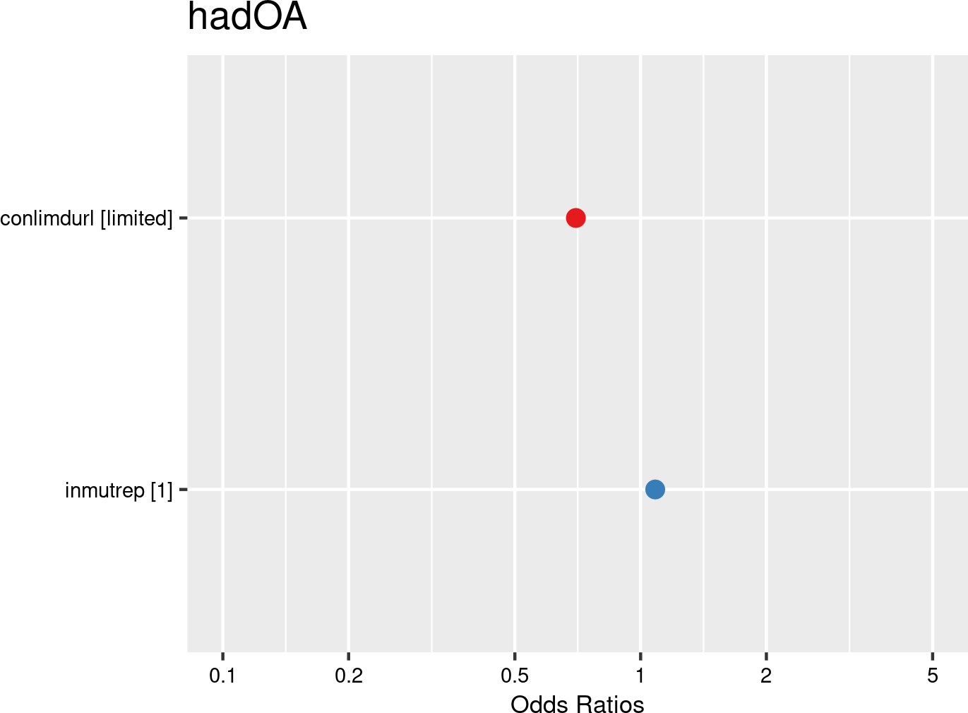

Contract type categories were introduced as fixed effects, and companies and employees as random effects. The model is based on data from employees with and without OAs from all mutual Liantis ESPP and PS customers. The model is adjusted for representativeness of the company (fixed effect inmutrep) regarding to sector, size and Flemish province.
According to Figure 3.106 (a) and Figure 3.106 (b), contract type does not significantly determine the likelihood of a reported OA being rejected by the insurer.
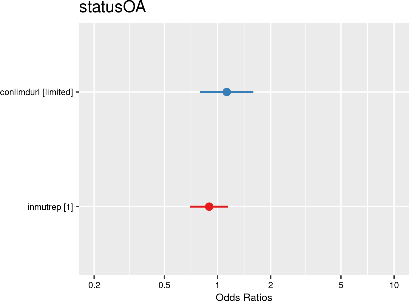

Contract type categories were introduced as fixed effects, and companies and employees as random effects. The model is based on data from employees notifying OAs from all mutual Liantis ESPP and PS customers. The model is adjusted for representativeness of the company (fixed effect inmutrep) regarding to sector, size and Flemish province.
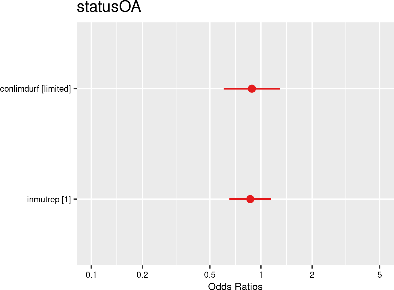

Contract type categories were introduced as fixed effects, and companies and employees as random effects. The model is based on data of all employees. The model is adjusted for representativeness of the company (fixed effect inmutrep) regarding to sector, size and Flemish province.
According to Figure 3.108 (a) and Figure 3.108 (b), workers with fixed-term contracts are less likely to have accepted commuting accidents compared to those with permanent contracts. This topic has not been extensively studied in scientific research yet. Possible explanations could include bias due to underreporting or differences in commuting distance or mode of transportation.
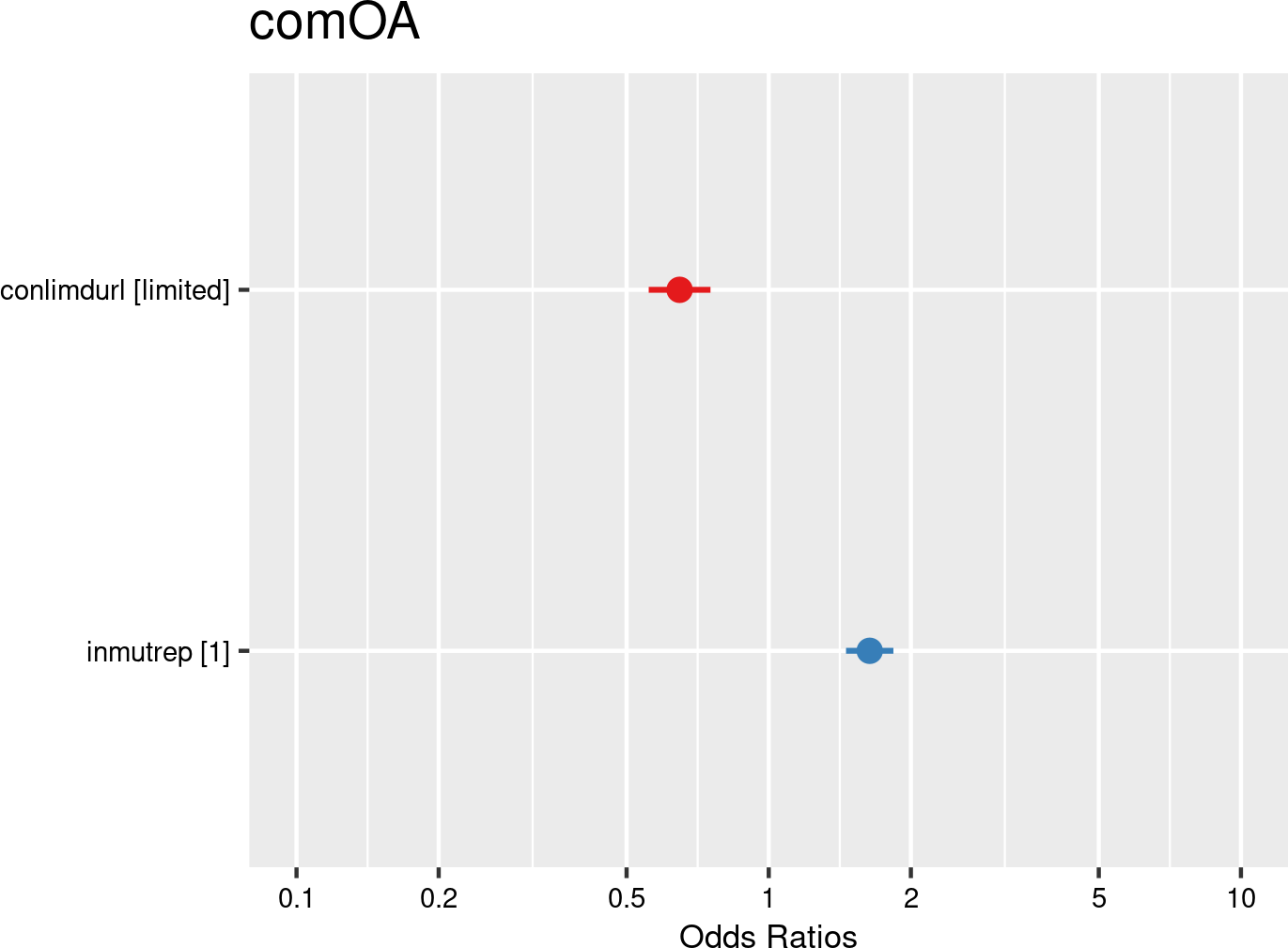

Contract type categories were introduced as fixed effects, and companies and employees as random effects. The model is based on data from employees with and without OAs from all mutual Liantis ESPP and PS customers. The model is adjusted for representativeness of the company (fixed effect inmutrep) regarding to sector, size and Flemish province.
Figure 3.109 (a) and Figure 3.109 (b) show the estimates for the relation between contract type categories and an accepted workplace OA. Once again, workers with fixed-term/limited contracts are less likely to experience accepted workplace accidents compared to those with permanent/unlimited contracts. This finding contradicts most previous research (Koranyi et al., 2018). Possible explanations for these inconsistencies include underreporting, uncertainty in how contract types are defined in the current analyses, or the specific jobs performed by workers with fixed-term contracts.
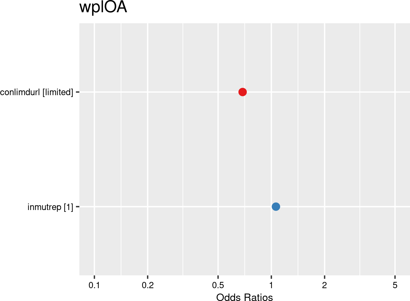

Contract type categories were introduced as fixed effects, and companies and employees as random effects. The model is based on data from employees with and without OAs from all mutual Liantis ESPP and PS customers. The model is adjusted for representativeness of the company (fixed effect inmutrep) regarding to sector, size and Flemish province.
Figure 3.110 (a) and Figure 3.110 (b) present a model estimating the frequency degree of OAs at the company level, in contrast to previous models that focused on individual employee accident probabilities. These figures indicate that a higher proportion of workers with a contract of unlimited duration significantly increases the frequency of OAs within a company. This is in line with the models above, which suggest that workers with a fixed-term contract have a lower chance of both commuting and workplace OAs. It is plausible that such contracts are more common in companies with higher risks for OAs. Additionally, underreporting of accidents in this specific group may also play a role in the explanation of these findings.
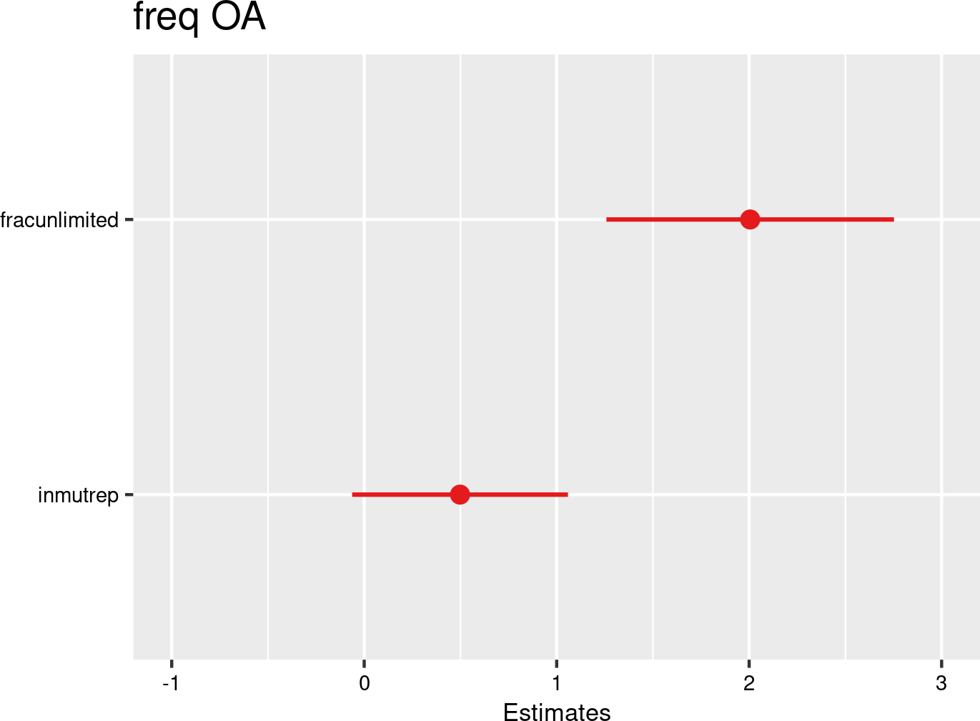

Contract type categories proportions were introduced as fixed effects, and companies as random effects. The model is based on data of all mutual Liantis ESPP and PS customers. The model is adjusted for representativeness of the company (fixed effect inmutrep) regarding to sector, size and Flemish province.
Figure 3.111 (a) and Figure 3.111 (b) present a model estimating the chance for an accepted accident being serious (according to the definition of the Belgian law). These figures indicate that contract type does not significantly determine whether an workplace OA is classified as serious. This contradicts earlier findings in the literature, which indicate that workers with temporary contracts are more likely to suffer severe injuries from workplace accidents compared to permanent workers (Picchio & Ours, 2016).
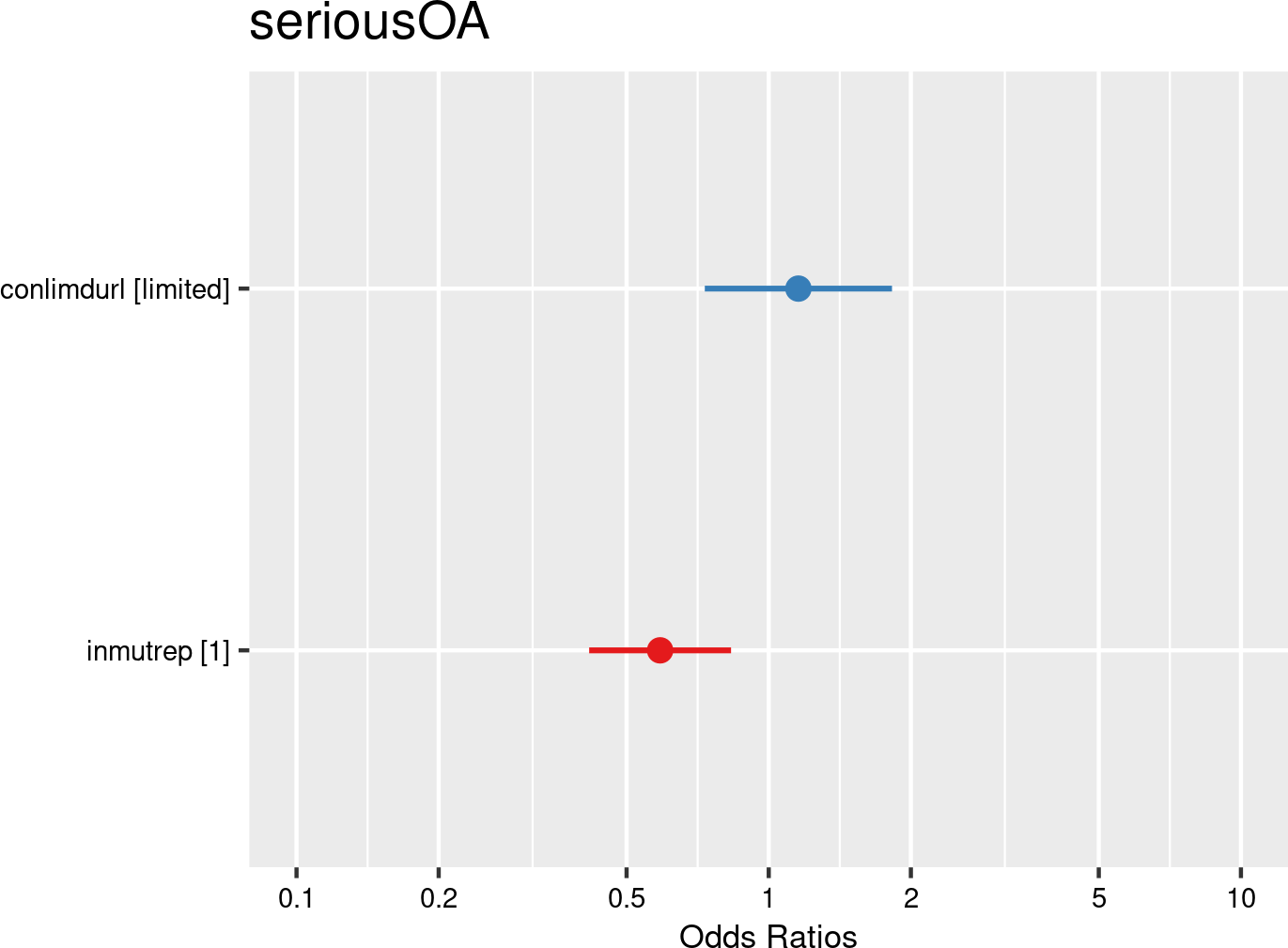

Contract type categories were introduced as fixed effects, and companies and employees as random effects. The model is based on data of all mutual Liantis ESPP and PS customers. The model is adjusted for representativeness of the company (fixed effect inmutrep) regarding to sector, size and Flemish province.
Figure 3.112 (a) and Figure 3.112 (b) show the results of a model assessing the relationship between contract type and the number of absenteeism days. These figures are based on absenteeism data from FEDRIS, while Figure 3.113 (a) and Figure 3.113 (b) present the same model using data from Liantis PS. The figures indicate that contract category is a significant factor in determining the validated number of absenteeism days due to OAs. The number of accepted days off decreases significantly for a contract with limited duration (e.g., 18% less days for a contract with limited duration).
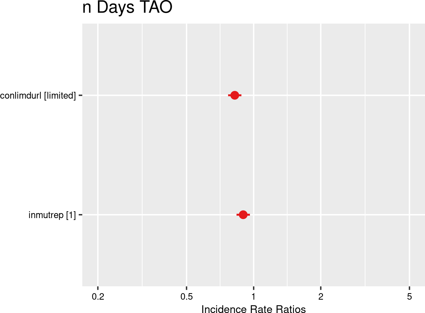

Contract type categories were introduced as fixed effects, and companies and employees as random effects. The model is based on data of all mutual Liantis ESPP and PS customers. The model is adjusted for representativeness of the company (fixed effect inmutrep) regarding to sector, size and Flemish province.
As mentioned above, Figure 3.113 (a) and Figure 3.113 (b) are the results of the model assessing the relation between contract type and number of absenteeism days related to the workplace accident, based on the Liantis PS data. Although the second model is based on a smaller sample size, findings aligns those of the model based on the FEDRIS absenteeims data, showing a lower number of absenteeism days for workers with a contract of limited duration. This again contradicts research that expect workers with fixed-term contracts having more absenteeism days due to OAs. However, the authors caution against using absenteeism as an outcome due to the risk of underreporting (Koranyi et al., 2018).
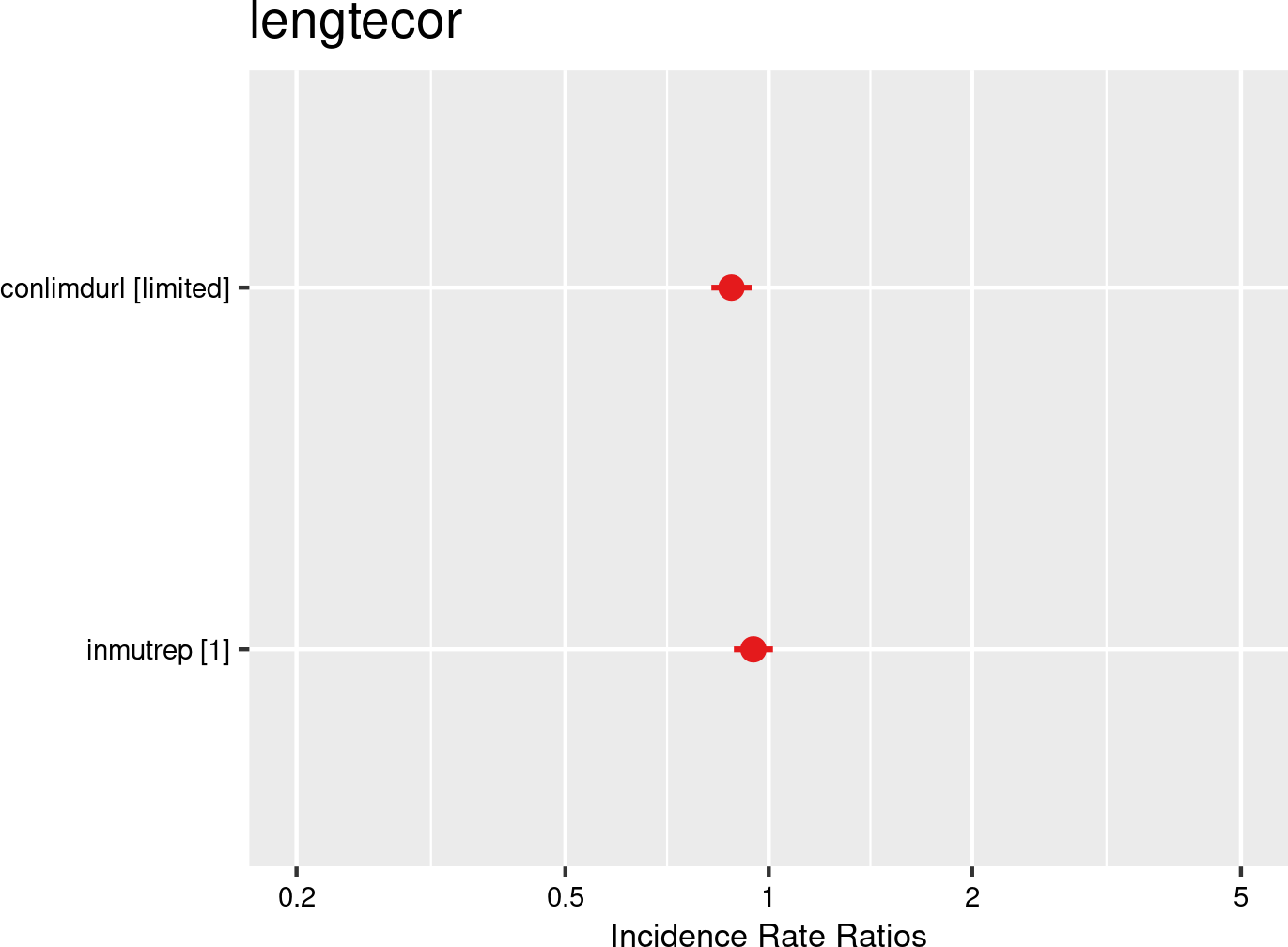

Contract type categories were introduced as fixed effects, and companies and employees as random effects. The model is based on data of all mutual Liantis ESPP and PS customers. The model is adjusted for representativeness of the company (fixed effect inmutrep) regarding to sector, size and Flemish province.
Figure 3.114 (a) and Figure 3.114 (b) show the results of a model evaluating the relationship between contract type and the direct wage cost of an OA. The findings indicate that contract type significantly impacts the direct wage cost for employers: contracts with limited duration incur lower costs compared to unlimited contracts. This aligns with expectations given the results of the former models regarding the relation with absenteeism.
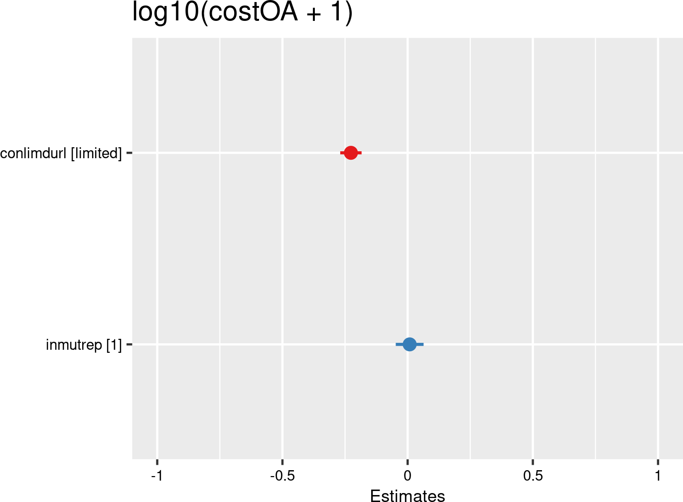

Contract type categories were introduced as fixed effects, and companies and employees as random effects. The model is based on data of all mutual Liantis ESPP and PS customers. The model is adjusted for representativeness of the company (fixed effect inmutrep) regarding to sector, size and Flemish province.
The next 4 figures (Figure 3.115 (a) and Figure 3.115 (b), Figure 3.116 (a) and Figure 3.116 (b)) are displaying the results of a model assessing the relation between proportion of workers within a contract type and the severity degree of a company, which is again a variable at the company level. In the first model (Figure 3.115 (a) and Figure 3.115 (b)), validated number of absenteeism days from FEDRIS were used, while the second model Figure 3.116 (a) and Figure 3.116 (b)) was based on the numbers of days off in the Liantis PS data. The results of both models indicate that a higher proportion of workers with a contract of unlimited duration significantly increases the severity degree within a company.
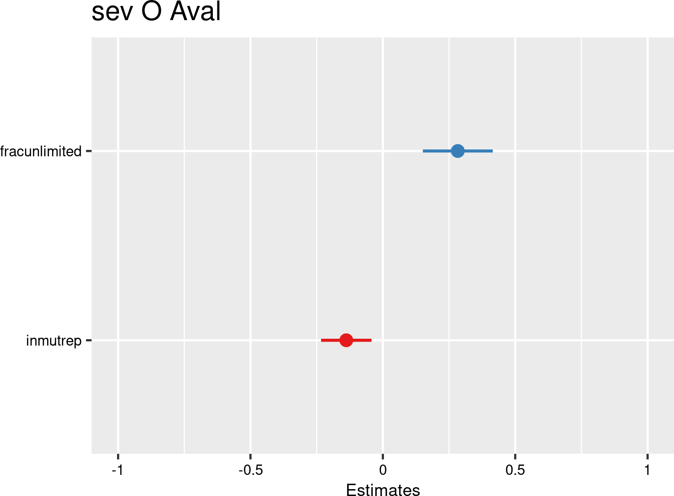

Contract type category proportions were introduced as fixed effects, and companies as random effects. The model is based on data of all mutual Liantis ESPP and PS customers. The model is adjusted for representativeness of the company (fixed effect inmutrep) regarding to sector, size and Flemish province.
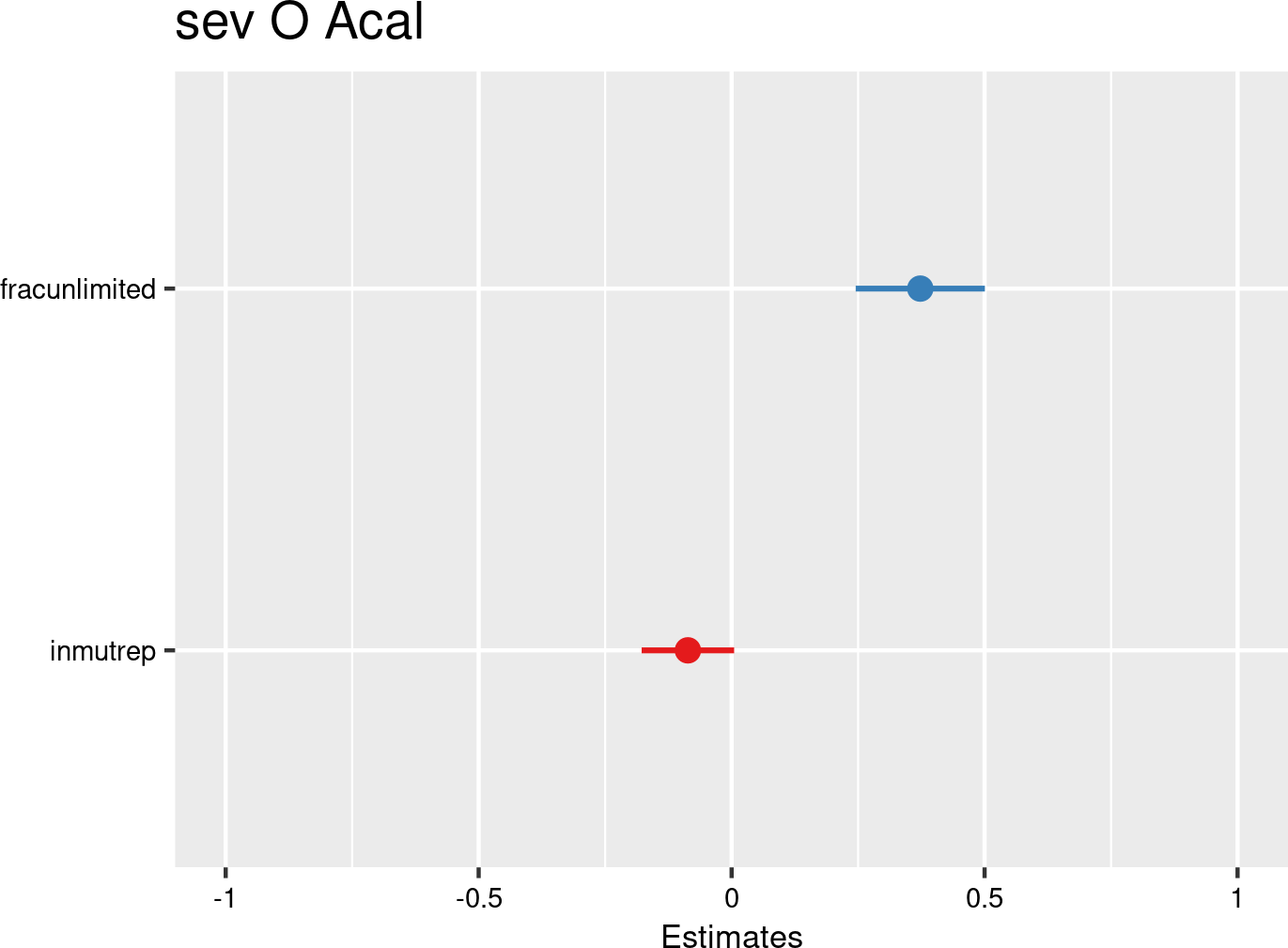

Contract type category proportions were introduced as fixed effects, and companies as random effects. The model is based on data of all mutual Liantis ESPP and PS customers. The model is adjusted for representativeness of the company (fixed effect inmutrep) regarding to sector, size and Flemish province.
3.4.2.3 Nature of the contract (full-time versus part-time employment)
3.4.2.3.1 Descriptives
The NSSO provides data on the nature of contracts in four categories: full-time, part-time, seasonal, or undetermined. Additionally, the FEDRIS statistical reports and notifications include information about the nature of contracts in three categories: full-time, part-time, and unknown.
Since Liantis PS data contains the number of hours an employee is expected to work per week, as well as the number of weekly hours an employee in the same role would work (the numerator and denominator of the so-called employment quotient), this quotient can be used as a proxy for full-time or part-time employment (\(\geq\) 1.00 is considered full-time, <1.00 as part-time, and unknown if the numerator and/or denominator are missing).
This allows us to categorize the nature of contracts in the same categories used in the FEDRIS reports and notifications. Given that the nature of contract categories is present in the notifications, the fit between the derived nature of the contract for an employee experiencing an OA can be compared with the corresponding nature of the contract classification in the accident notification.
According to Figure 3.117, the contract categories in Liantis PS data and FEDRIS data are quite comparable. This indicates that the contract categories derived from Liantis PS data might align well with those in FEDRIS data, making them suitable for further analysis. The combined accuracy is 85%.
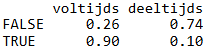
In the next 6 tables, an overview of all (accepted) OAs (Table 3.78 and Table 3.79), the commuting OAs (Table 3.80 and Table 3.81) and the workplace OAs (Table 3.82 and Table 3.83) are given.
In the first table ((Table 3.78, Table 3.80 and Table 3.82), the absolute numbers are provided stratified per contract category, next to the total number of employees, as available in the Liantis database.
In the second table (Table 3.79, Table 3.81 and Table 3.83), the relative numbers of the OAs per contract category are provided as percentages.
From the table Table 3.79, it can be noticed that full-time workers account for 65% of the employees within Liantis customers, while they account for about 75% of the employees within the notifications. For the commuting OAs (Table 3.81), these percentage are somewhat more balanced.
all accepted occupational accidents
| name | rszall | rszpriv | liaall | fedrisall | totalnot | totalnotmut | totalnotrepmutflan |
|---|---|---|---|---|---|---|---|
| fulltime | 96371160 | NA | 11797777 | 0 | 119078 | 33177 | 13717 |
| parttime | 51035685 | NA | 6257299 | 0 | 40305 | 12959 | 7190 |
| seasonal | 5504361 | NA | NA | NA | NA | NA | NA |
| unknown | 256936 | NA | 790 | 0 | 35836 | 15099 | 5123 |
| name | percrszall | percrszpriv | percliaall | percfedrisall | perctotalnot | perctotalnotmut | perctotalnotrepmutflan |
|---|---|---|---|---|---|---|---|
| fulltime | 65.4 | NA | 65.3 | NaN | 74.7 | 71.9 | 65.6 |
| parttime | 34.6 | NA | 34.7 | NaN | 25.3 | 28.1 | 34.4 |
| seasonal | NA | NA | NA | NA | NA | NA | NA |
| unknown | NA | NA | NA | NA | NA | NA | NA |
commuting accepted occupational accidents
| name | rszall | rszpriv | liaall | fedrisall | totalnot | totalnotmut | totalnotrepmutflan |
|---|---|---|---|---|---|---|---|
| fulltime | 96371160 | NA | 11797777 | 0 | 15927 | 4045 | 1946 |
| parttime | 51035685 | NA | 6257299 | 0 | 7972 | 2581 | 1391 |
| seasonal | 5504361 | NA | NA | NA | NA | NA | NA |
| unknown | 256936 | NA | 790 | 0 | 4488 | 1973 | 775 |
| name | percrszall | percrszpriv | percliaall | percfedrisall | perctotalnot | perctotalnotmut | perctotalnotrepmutflan |
|---|---|---|---|---|---|---|---|
| fulltime | 65.4 | NA | 65.3 | NaN | 66.6 | 61 | 58.3 |
| parttime | 34.6 | NA | 34.7 | NaN | 33.4 | 39 | 41.7 |
| seasonal | NA | NA | NA | NA | NA | NA | NA |
| unknown | NA | NA | NA | NA | NA | NA | NA |
workplace accepted occupational accidents
| name | rszall | rszpriv | liaall | fedrisall | totalnot | totalnotmut | totalnotrepmutflan |
|---|---|---|---|---|---|---|---|
| fulltime | 96371160 | NA | 11797777 | 691920 | 103151 | 29132 | 11771 |
| parttime | 51035685 | NA | 6257299 | 243576 | 32333 | 10378 | 5799 |
| seasonal | 5504361 | NA | NA | NA | NA | NA | NA |
| unknown | 256936 | NA | 790 | 191571 | 31348 | 13126 | 4348 |
| name | percrszall | percrszpriv | percliaall | percfedrisall | perctotalnot | perctotalnotmut | perctotalnotrepmutflan |
|---|---|---|---|---|---|---|---|
| fulltime | 65.4 | NA | 65.3 | 74 | 76.1 | 73.7 | 67 |
| parttime | 34.6 | NA | 34.7 | 26 | 23.9 | 26.3 | 33 |
| seasonal | NA | NA | NA | NA | NA | NA | NA |
| unknown | NA | NA | NA | NA | NA | NA | NA |
3.4.2.3.2 Models
The following Table 3.84 summarizes the results of the models assessing the relationship between contract and the several outcomes related to OAs. Below the table, details are provided about the data used for the analyses. The results of the nine models are then presented both in a table and graphically.
| catnature | chance to notify | chance on refusal | chance commuting | chance workplace | freq degree | chance serious | nDays TAO V/C | cost | sev degree V/C |
|---|---|---|---|---|---|---|---|---|---|
| Part-time | REF | REF/> | REF | REF | rank def | REF | </ns | < | rank def |
| Full-time | > | </REF | ns | > | > | > | REF | REF | >/> |
| occur | accept | occur | occur | occur | severe | severe | severe | severe | |
| empl | empl | empl | empl | comp | empl | empl | empl | comp | |
| c/w all | c/w ref | c acc | w acc | w acc | w acc | w acc | w acc | w acc |
- occur: data include all workers, chance for occurrence is calculated for the outcome
- accept: data include only workers with a notification of OA
- severe: data include only workers with an accepted OA
- c/w all: commuting and workplace accidents, including refused and accidents without decisions
- c/w ref: accepted or refused commuting and workplace accidents
- c acc: accepted commuting accidents
- w acc: accepted workplace accidents
- empl: the outcome is situated at the individual level
- comp: the outcome is situated at the company level
- nDaysTAO: number of days absenteeism related to the OA
- V/C: Validated number of days (available from FEDRIS) / Calculated number of days (based on the Liantis PS data)
Nature of the contract (full-time versus part-time employment) and occupational accidents
- Full-time workers have a higher chance to report an occupational accident (and have a higher chance for both an accepted commuting as an accepted workplace occupational accident).
- Part-time workers seem to show a higher chance that a reported occupational accident is refused by an insurer. A multivariable model should confirm this finding.
- Full-time workers have a higher chance for an occupational accident being serious in comparison with part-time workers.
- Inconsistent results were found for the relation between nature of contract type and number of absenteeism days.
- A higher proportion of full-time workers significantly increases the frequency and severity degree within a company.
Figure 3.118 (a) and Figure 3.118 (b) illustrate that workers with a full-time contract have 55% more chance of reporting an OA (both commuting and workplace accidents) compared to the category with a part-time contract, even after accounting for significant differences in company representativeness. It should be noted that in literature, findings are inconsistent: some literature reports higher likelihood for OAs for full-time workers (Alamgir et al., 2008; Picchio & Ours, 2017), while other findings suggest the opposite (Alali et al., 2016).
It is possible that part-time workers are less familiar with workplace routines, which may increase the risk of accidents, although they may be less likely to report them. Moreover, a substantial body of literature treats part-time status as a proxy for fixed-term or precarious contracts, which may also be concentrated in specific sectors.
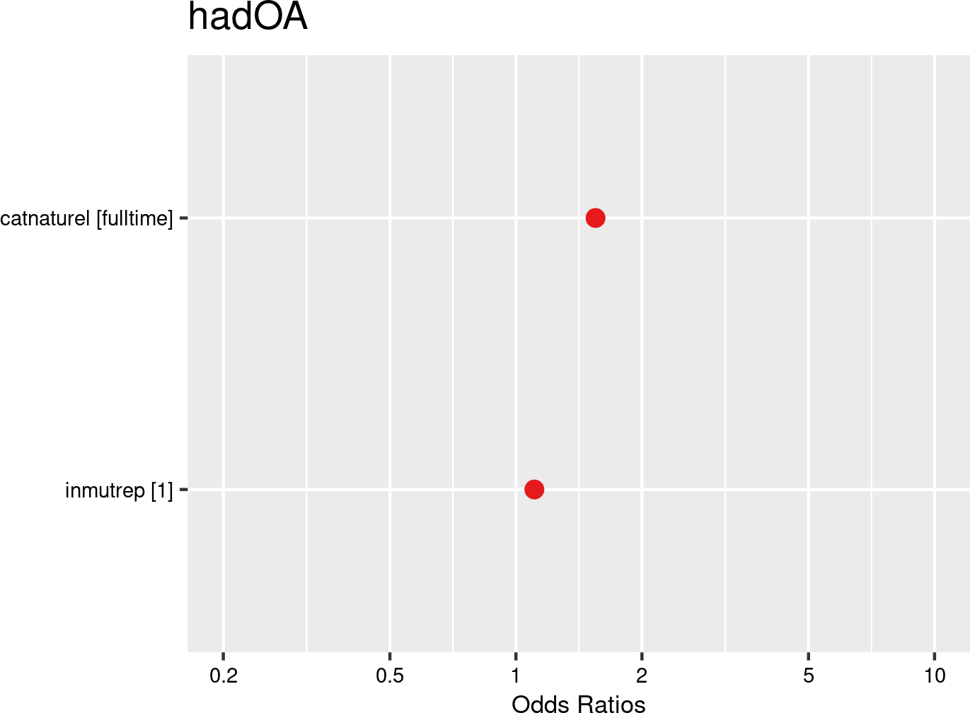

Nature of the contract categories were introduced as fixed effects, and companies and employees as random effects. The model is based on data from employees with and without OAs from all mutual Liantis ESPP and PS customers. The model is adjusted for representativeness of the company (fixed effect inmutrep) regarding to sector, size and Flemish province.
According to Figure 3.119 (a) and Figure 3.119 (b) (Liantis PS data) and Figure 3.120 (a) and Figure 3.120 (b) (Fedris notification data), the workers with a full-time contract have a lower chance for a reported OA being refused by the insurer. This may be because part-time workers are less familiar with the procedures for reporting OAs, potentially leading to late reports or incorrect procedures, which makes the claims more disputable (Kreshpaj et al., 2021).
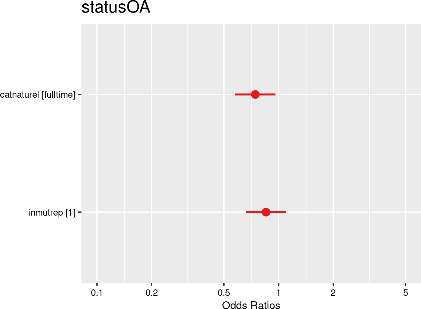

Nature of the contract categories were introduced as fixed effects, and companies and employees as random effects. The model is based on data from employees notifying OAs from all mutual Liantis ESPP and PS customers. The model is adjusted for representativeness of the company (fixed effect inmutrep) regarding to sector, size and Flemish province.
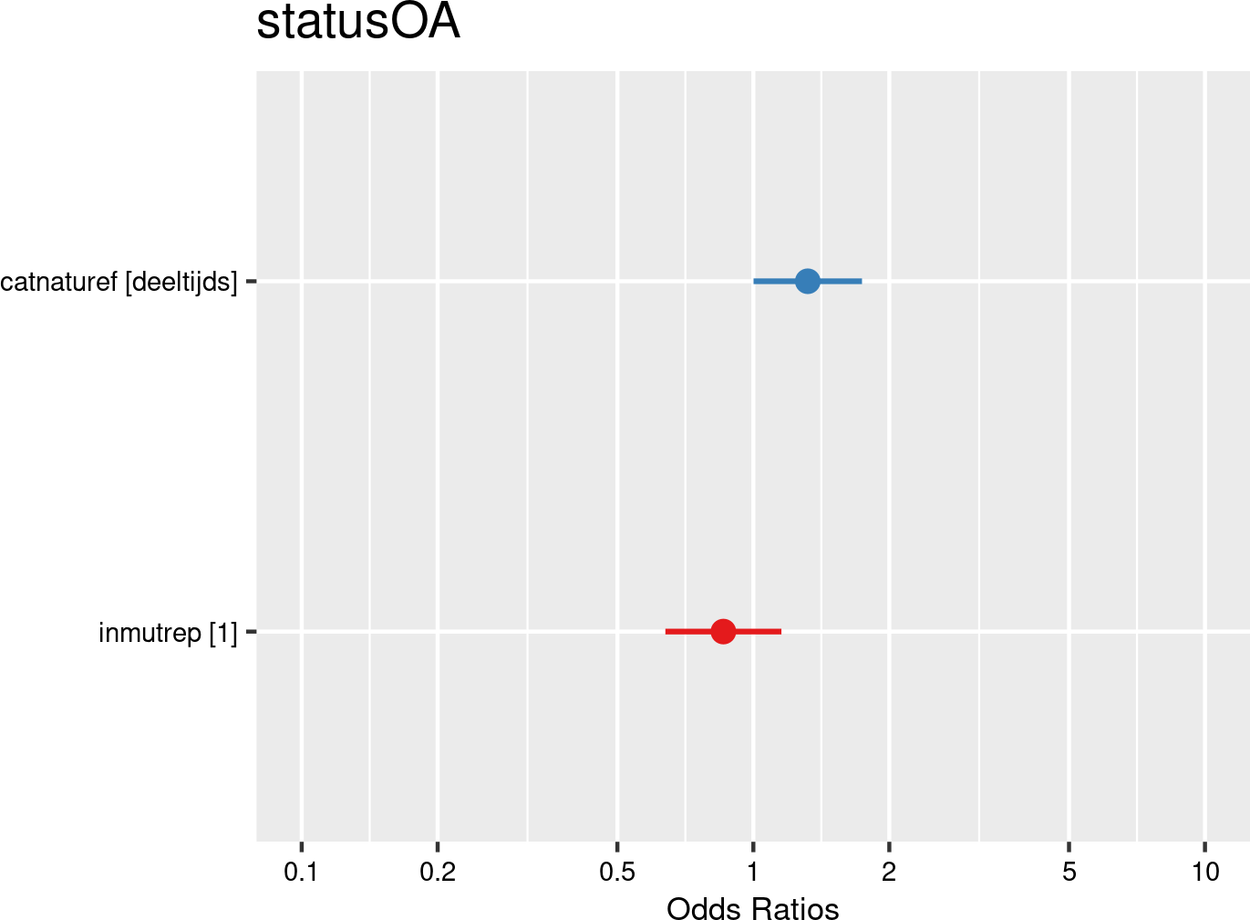

Contract categories were introduced as fixed effects, and companies and employees as random effects. The model is based on data from employees notifying OAs from all mutual Liantis ESPP and PS customers. The model is adjusted for representativeness of the company (fixed effect inmutrep) regarding to sector, size and Flemish province.
According to Figure 3.121 (a) and Figure 3.121 (b), full-time employment does not seem to determine the chance of experiencing an accepted commuting accident. We are not aware of specific studies examining this relationship (more commonly studied variables include commuting time and work-home distance).
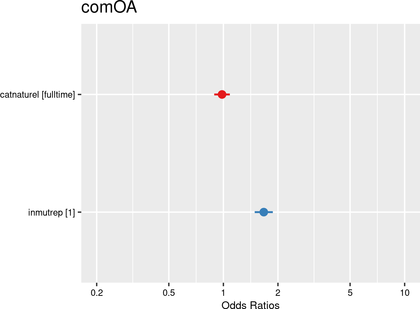

Nature of the contract categories were introduced as fixed effects, and companies and employees as random effects. The model is based on data from employees with and without OAs from all mutual Liantis ESPP and PS customers. The model is adjusted for representativeness of the company (fixed effect inmutrep) regarding to sector, size and Flemish province.
Figure 3.122 (a) and Figure 3.122 (b) show the estimates for the relation between contract categories and an accepted workplace OA. Full-time workers have a higher likelihood (65% more than part-time workers) for experiencing an accepted workplace OA.
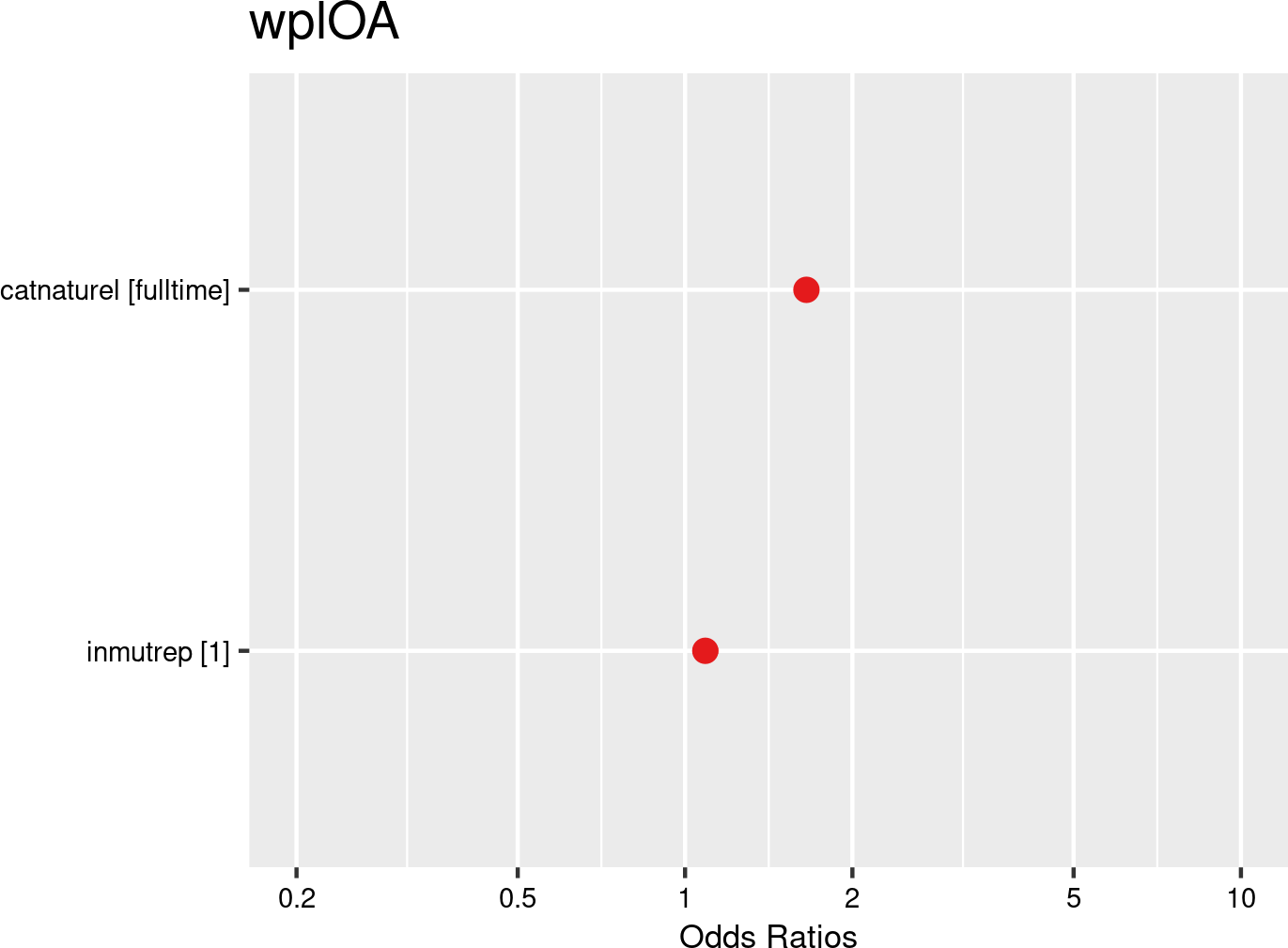

Nature of the categories were introduced as fixed effects, and companies and employees as random effects. The model is based on data from employees with and without OAs from all mutual Liantis ESPP and PS customers. The model is adjusted for representativeness of the company (fixed effect inmutrep) regarding to sector, size and Flemish province.
Figure 3.123 (a) and Figure 3.123 (b) present a model estimating the frequency degree of OAs at the company level, in contrast to previous models that focused on individual employee accident probabilities. These figures indicate that a higher proportion of full-time workers significantly increases the frequency of OAs within a company.
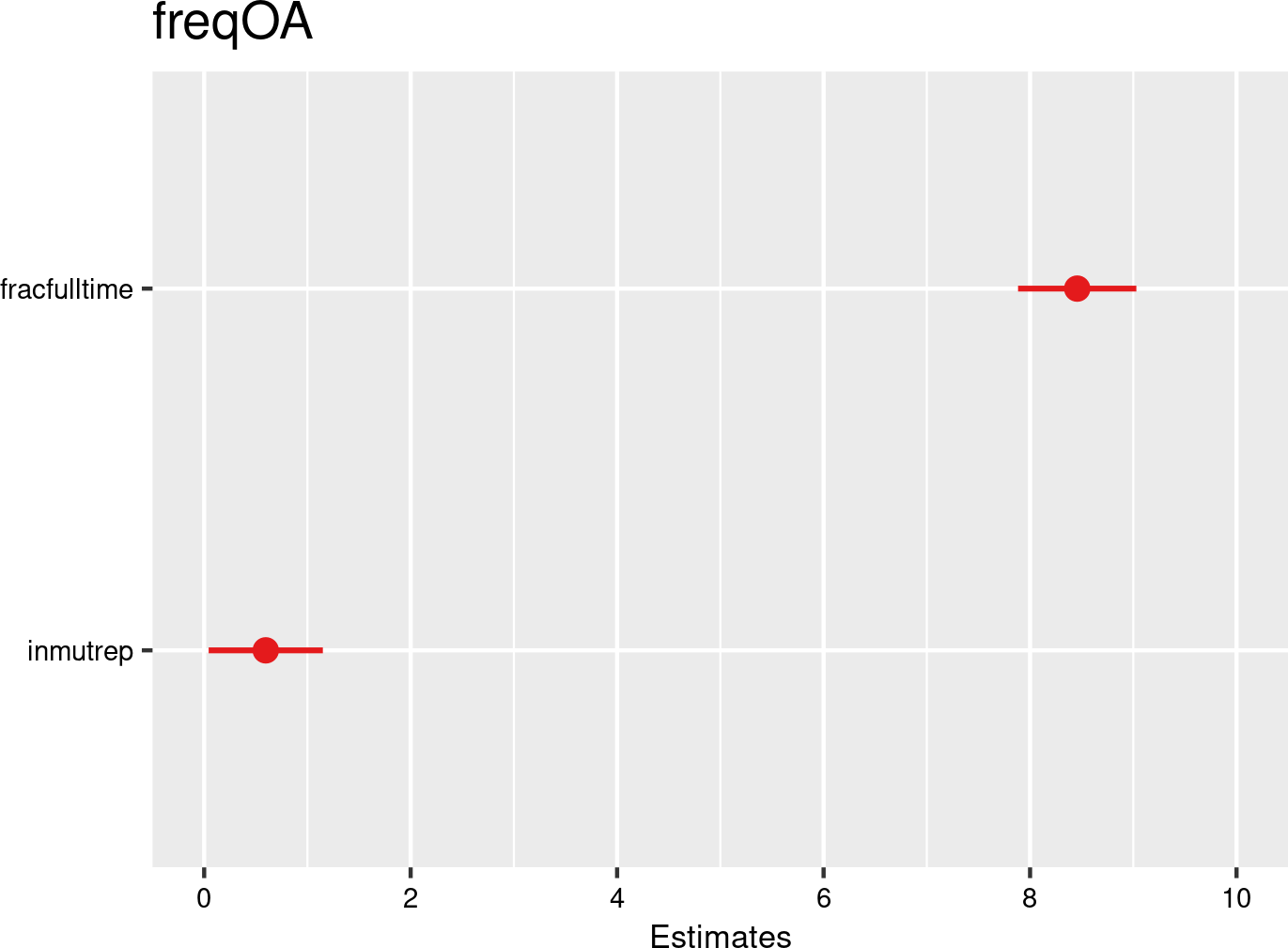

Nature of the contract categories proportions were introduced as fixed effects, and companies as random effects. The model is based on data of all mutual Liantis ESPP and PS customers. The model is adjusted for representativeness of the company (fixed effect inmutrep) regarding to sector, size and Flemish province.
Figure 3.124 (a) and Figure 3.124 (b) present a model estimating the chance for an accepted accident being serious (according to the definition of the Belgian law). These figures indicate that the nature of the contract category does significantly determine whether an workplace OA is classified as serious: for full-time workers, the chance for an OA being classified as serious is 81% higher than for part-time workers.
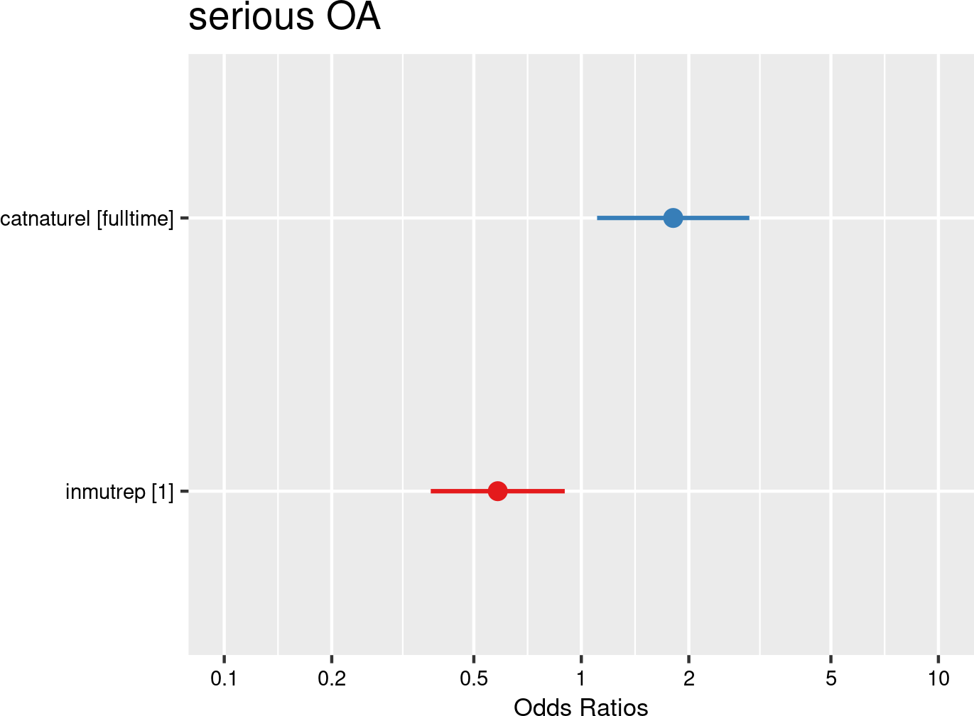

Nature of the contract categories were introduced as fixed effects, and companies and employees as random effects. The model is based on data of all mutual Liantis ESPP and PS customers. The model is adjusted for representativeness of the company (fixed effect inmutrep) regarding to sector, size and Flemish province.
Figure 3.125 (a) and Figure 3.125 (b) show the results of a model assessing the relationship between contract category and the number of absenteeism days. These figures are based on absenteeism data from FEDRIS, while Figure 3.126 (a) and Figure 3.126 (b) present the same model using data from Liantis PS. The figures indicate that contract category is a significant factor in determining the validated number of absenteeism days due to OAs. The number of accepted days off decreases significantly for a part-time contract (e.g., 6% less days for a part-time contract).
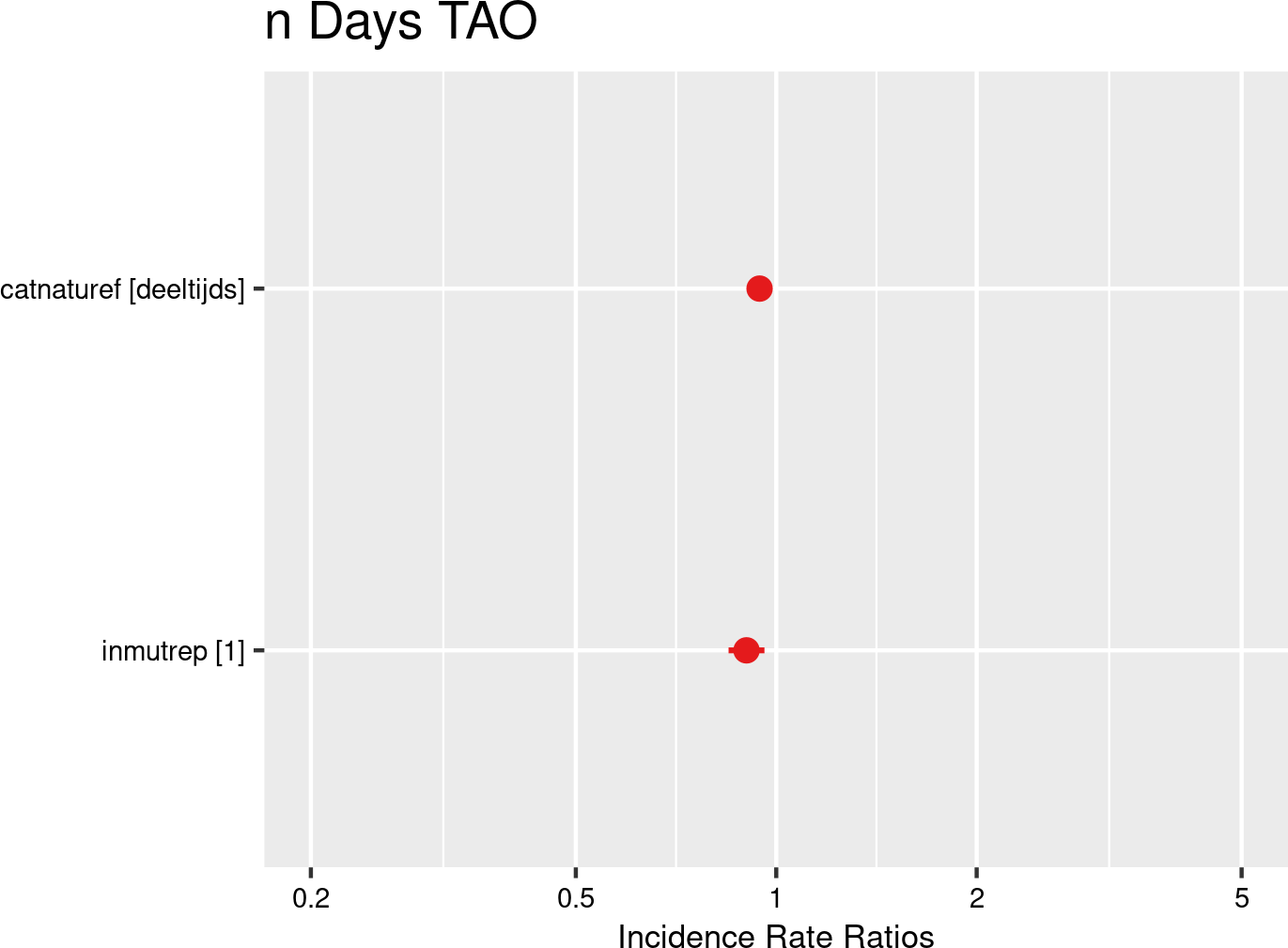

Nature of the contract categories were introduced as fixed effects, and companies and employees as random effects. The model is based on data of all mutual Liantis ESPP and PS customers. The model is adjusted for representativeness of the company (fixed effect inmutrep) regarding to sector, size and Flemish province.
As mentioned above, Figure 3.126 (a) and Figure 3.126 (b) are the results of the model assessing the relation between contract category and number of absenteeism days related to the workplace accident, based on the Liantis PS data. The results conflict with those of the previous model. They indicate that part-time workers have slightly more accepted days off than full-time workers, although the results are not significant. These inconsistent findings may be due to differences in the study populations between the Liantis PS data and the FEDRIS absenteeism data. The Liantis PS dataset is considerably smaller, with fewer than half the number of employers and less than one-fifth the number of employees.
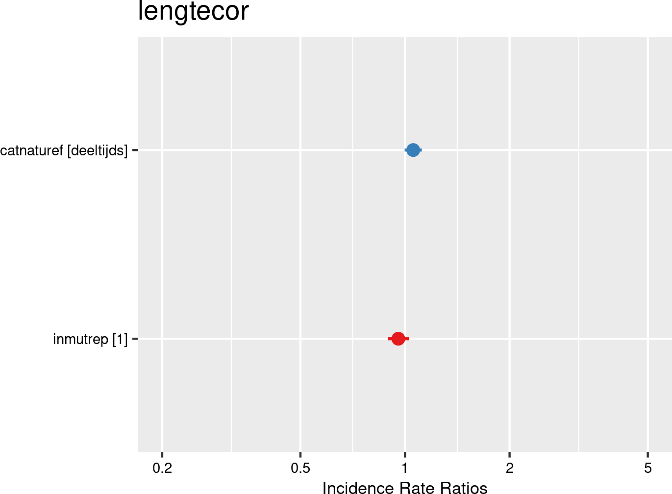

Contract categories were introduced as fixed effects, and companies and employees as random effects. The model is based on data of all mutual Liantis ESPP and PS customers. The model is adjusted for representativeness of the company (fixed effect inmutrep) regarding to sector, size and Flemish province.
Figure 3.127 (a) and Figure 3.127 (b) show the results of a model evaluating the relationship between contract category and the direct wage cost of an OA. The findings indicate that contract type significantly impacts the direct wage cost for employers: part-time contracts incur lower costs compared to full-time contracts, which aligns with expectations.


Nature of the contract categories were introduced as fixed effects, and companies and employees as random effects. The model is based on data of all mutual Liantis ESPP and PS customers. The model is adjusted for representativeness of the company (fixed effect inmutrep) regarding to sector, size and Flemish province.
The next 4 figures (Figure 3.128 (a) and Figure 3.128 (b), Figure 3.129 (a) and Figure 3.129 (b)) are displaying the results of a model assessing the relation between proportion of workers within a contract category and the severity degree of a company, which is again a variable at the company level. In the first model (Figure 3.128 (a) and Figure 3.128 (b)), validated number of absenteeism days from FEDRIS were used, while the second model (Figure 3.129 (a) and Figure 3.129 (b)) was based on the numbers of days off in the Liantis PS data. The results of both models indicate that a higher proportion of full-time workers significantly increases the severity level within a company.
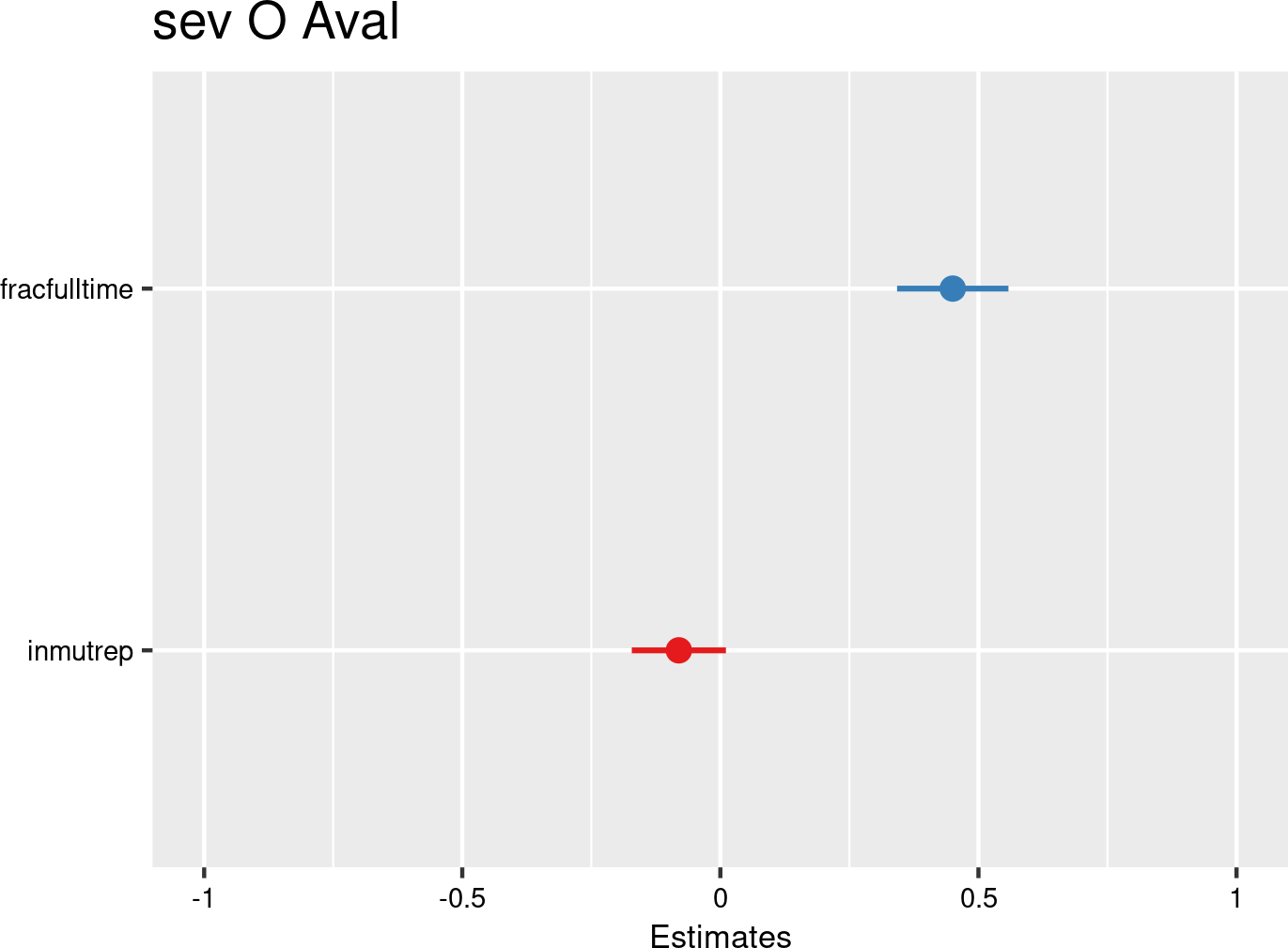

Nature of the contract category proportions were introduced as fixed effects, and companies as random effects. The model is based on data of all mutual Liantis ESPP and PS customers. The model is adjusted for representativeness of the company (fixed effect inmutrep) regarding to sector, size and Flemish province.
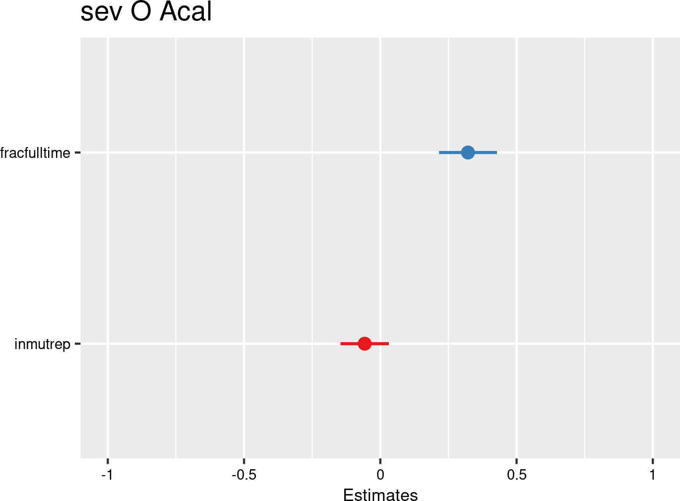

Nature of the contract category proportions were introduced as fixed effects, and companies as random effects. The model is based on data of all mutual Liantis ESPP and PS customers. The model is adjusted for representativeness of the company (fixed effect inmutrep) regarding to sector, size and Flemish province.
3.4.2.4 Working in shifts and long working hours
Data Quality Alert: working in shifts
- Liantis ESPP risk codes for night and shift work are available but not always explicitly negatively validated
- Many assumptions would have to be made to use the available information in modelling
Within Liantis, no systematically maintained variables related to working in shifts are currently available that would allow for investigation of a potential association with occupational accidents. Similarly, the FEDRIS notification data does not include any variables related to working in shifts. As a result, no further analyses or modelling efforts were undertaken in relation to working in shifts.
Data Quality Alert: long working hours
- To our knowledge, no data quantitative data on long working hours is at this moment easily accessible in the Liantis ESPP or PS data
- In the FEDRIS occupational accident data, information on the duration of the shift is indirectly present and be calculated (in 60% of the notifications) from the difference between the end and start of the work shift (see Section 2.7.2.7)
- Many assumptions would have to be made to use the available information in modelling
Within Liantis, no systematically maintained variables related to long working hours are currently available that would allow for investigation of a potential association with occupational accidents. Additionally, the FEDRIS notification data do not include detailed quantitative information on the length of shifts. As a result, no further analyses or modelling efforts were undertaken in relation to long working hours.
3.4.2.5 Hazards in work system
3.4.2.5.1 Usual professional work activity
Data Quality Alert: usual professional work activity
- Liantis (neither ESPP nor PS) does not have information on the frequencies with which all employees are exposed to work activities deviating from the usual professional work activity like FEDRIS describes in the context of occupational accidents
- Information on deviation of the usual professional work activity is only present in occupational accident notifications received via FEDRIS (see Section 2.7.2.10)
Within Liantis, no systematically maintained variables related to deviations from usual professional work activities are currently available that would allow for investigation of a potential association with occupational accidents. As a result, no further analyses or modelling efforts were undertaken in relation to the usual professional work activity.
3.4.2.5.2 Specific activity
Data Quality Alert: specific activity
- Liantis (neither ESPP nor PS) does not have information on the frequencies with which all employees exhibit specific activities or work processes in a structured way like FEDRIS or European Statistics on Accidents at Work (ESAW) describe in the context of occupational accidents
- Information on specific activity is only present in occupational accident notifications received via FEDRIS (see Section 2.7.2.8)
Within Liantis, no systematically maintained variables related to specific activities are currently available that would allow for investigation of a potential association with occupational accidents. As a result, no further analyses or modelling efforts were undertaken in relation to the specific activity.
3.4.2.5.3 Type of workstation
Data Quality Alert: type of workstation
- Liantis (neither ESPP nor PS) does not have information on the frequencies with which all employees exhibit activities at a specific type of workstation in a structured way like FEDRIS or ESAW describe in the context of occupational accidents
- Information on type of workstation is only present in occupational accident notifications received via FEDRIS (see Section 2.7.2.9)
Within Liantis, no systematically maintained variables related to type of workstation are currently available that would allow for investigation of a potential association with occupational accidents. As a result, no further analyses or modelling efforts were undertaken in relation to type of workstation.
3.4.2.5.4 Risks (ESPP)
Data Quality Alert: risks
- Liantis ESPP assigns risk codes (see Section 2.11) to employees. However, assumptions must be made to use these risk codes in statistical modelling.
- When a certain risk is present, the corresponding risk code is assigned. Positive or negative validation is not performed monthly, so we assume the employee is exposed to the risk only if the risk code is valid.
- Since there are more than 40 risk code groups, with large variation in both the number of codes and their frequency of use (some are assigned very often, others almost never), our models struggled to converge. Many risk code groups had to be excluded to achieve convergence.
- Therefore, we chose to focus only on comparing univariable models for the likelihood of experiencing an accepted commuting versus an accepted workplace OA.
Only screen work is significantly associated with a lower likelihood of workplace occupational accidents
- Most predictors in the univariable models show wide confidence intervals and non-significant p-values, indicating low statistical power and high uncertainty.
- Screen work is the only statistically significant predictor for workplace occupational accidents, showing a protective effect (OR = 0.35, p = 0.001); no predictors were significant for commuting occupational accidents.
- The safety function variable shows a non-significant trend: possibly protective for commuting OA (OR = 0.55) and slightly risk-enhancing for workplace OA (OR = 1.23), suggesting role-specific dynamics.
- Model quality is dominated by random effects (conditional R² and ICC > 0.96), meaning contextual factors explain most of the variance, while fixed-effect predictors contribute very little (marginal R² < 0.01).
- Because of the low added value of the risk code predictors in these univariable models, the convergence problems, and the risk of further waterfall loss of cases, multivariable models using the risk code predictor will not be pursued further.
In Figure 3.130, a graphical representation of the commuting and workplace model is provided.
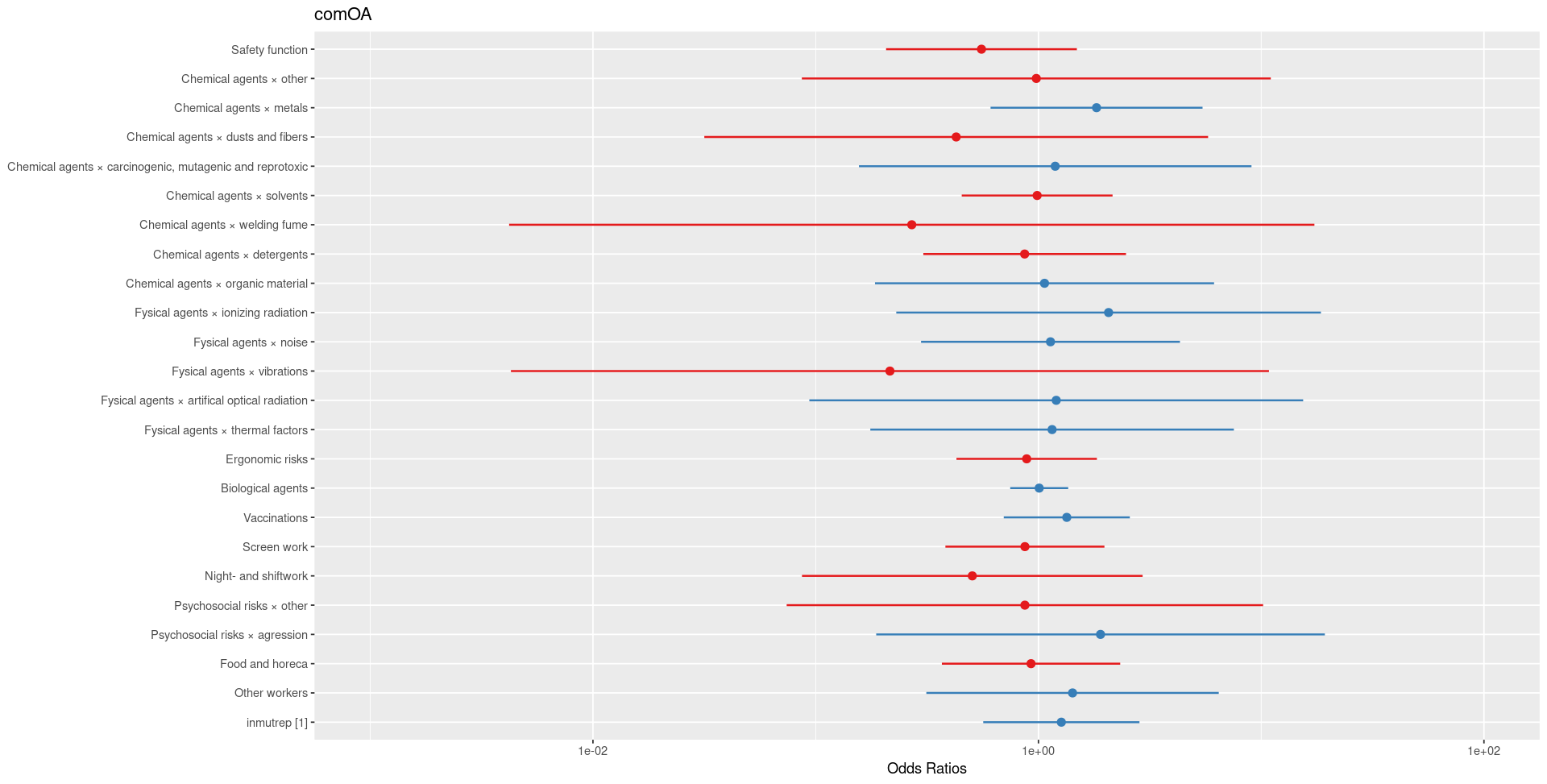
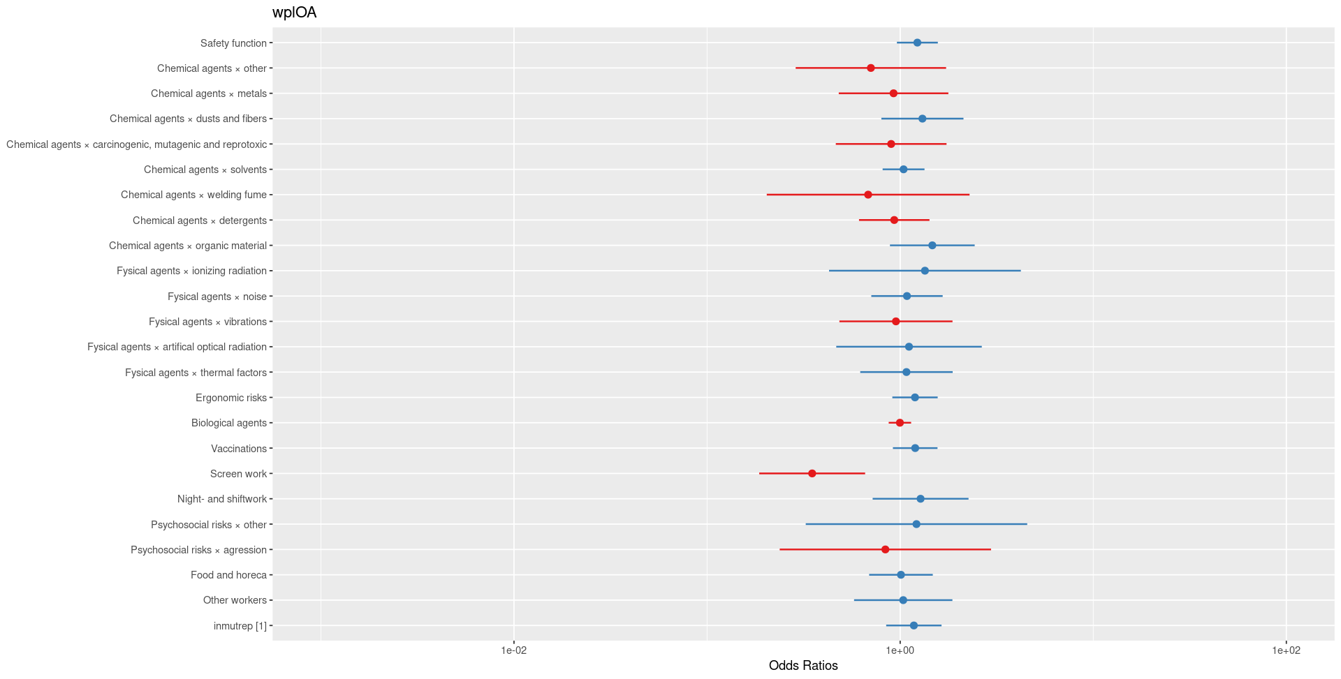
Both models are shown side-by-side in Figure 3.131 for easier comparison. The explained variance is very similar in both models, with conditional R² values above 0.96 and marginal R² values below 0.01. This indicates that the random effects (company and employee) explain most of the variance, while the fixed effects (risk codes) contribute very little. Screen work is the only risk code showing a statistically significant association, specifically a protective effect against workplace OA (OR = 0.35, p = 0.001). No risk codes are significantly associated with a higher likelihood of commuting or workplace OA in our ten-year dataset.

3.4.3 Organisation related factors
3.4.3.1 Work location
3.4.3.1.1 Descriptives
Both NSSO and FEDRIS provide statistics on the work location of the employee (Province). From Liantis PS data it is also possible to derive the Province of the employer through the postal code of an employer adress. The notification in many cases also contains the postal code of the employer. Since this information is also present in the notification information passed through to Liantis, the fit between the derived work location of the employer of an employee experiencing an OA can be compared with the corresponding work location classification in the original notification of the accident.
From Figure 3.132 we learn that the work location provinces derived from Liantis PS data and FEDRIS data are highly comparable when both are available. The correlation between the two datasets is >99%. This suggests that the work provinces derived from Liantis PS data align well with those in FEDRIS data, making them suitable for further analysis.
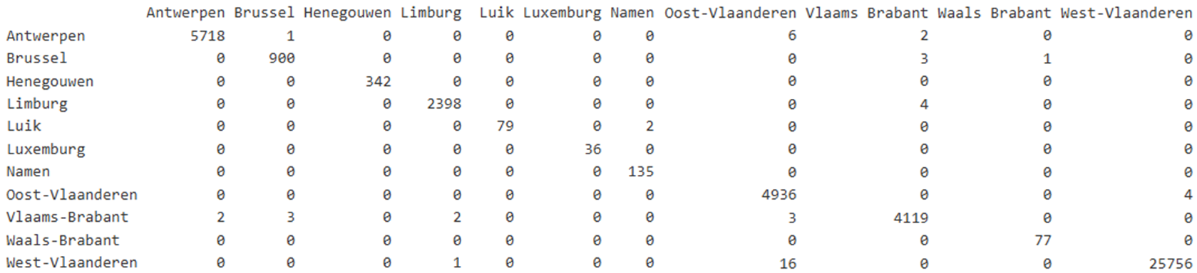
all accepted occupational accidents
| province | rszall | rszpriv | liaall | fedrisall | totalnot | totalnotmut | totalnotrepmutflan |
|---|---|---|---|---|---|---|---|
| Antwerpen | NA | NA | 2567346 | 246074 | 23472 | 7938 | 3897 |
| Brussel | NA | NA | 577831 | 223134 | 6641 | 1821 | 149 |
| Henegouwen | NA | NA | 97651 | 102403 | 6010 | 967 | NA |
| Limburg | NA | NA | 1262033 | 98040 | 9081 | 5512 | 1585 |
| Luik | NA | NA | 42563 | 91345 | 20099 | 195 | NA |
| Luxemburg | NA | NA | 11524 | 17764 | 1268 | 56 | NA |
| Namen | NA | NA | 49528 | 40733 | 7799 | 263 | NA |
| Oost-Vlaanderen | NA | NA | 2078211 | 159068 | 31016 | 6759 | 3540 |
| Unknown | NA | NA | 1465100 | 29171 | 13324 | 71 | 10 |
| Vlaams Brabant | NA | NA | 1803293 | 123953 | 10710 | 5343 | 2380 |
| Waals Brabant | NA | NA | 61516 | 28287 | 1574 | 256 | NA |
| West-Vlaanderen | NA | NA | 8039270 | 193405 | 64225 | 32054 | 14469 |
| province | percrszall | percrszpriv | percliaall | percfedrisall | perctotalnot | perctotalnotmut | perctotalnotrepmutflan |
|---|---|---|---|---|---|---|---|
| Antwerpen | NA | NA | 14.22 | 18.18 | 12.02 | 12.96 | 14.97 |
| Brussel | NA | NA | 3.20 | 16.49 | 3.40 | 2.97 | 0.57 |
| Henegouwen | NA | NA | 0.54 | 7.57 | 3.08 | 1.58 | NA |
| Limburg | NA | NA | 6.99 | 7.24 | 4.65 | 9.00 | 6.09 |
| Luik | NA | NA | 0.24 | 6.75 | 10.30 | 0.32 | NA |
| Luxemburg | NA | NA | 0.06 | 1.31 | 0.65 | 0.09 | NA |
| Namen | NA | NA | 0.27 | 3.01 | 4.00 | 0.43 | NA |
| Oost-Vlaanderen | NA | NA | 11.51 | 11.75 | 15.89 | 11.04 | 13.60 |
| Unknown | NA | NA | 8.11 | 2.16 | 6.83 | 0.12 | 0.04 |
| Vlaams Brabant | NA | NA | 9.99 | 9.16 | 5.49 | 8.73 | 9.14 |
| Waals Brabant | NA | NA | 0.34 | 2.09 | 0.81 | 0.42 | NA |
| West-Vlaanderen | NA | NA | 44.52 | 14.29 | 32.90 | 52.35 | 55.59 |
commuting accepted occupational accidents
| province | rszall | rszpriv | liaall | fedrisall | totalnot | totalnotmut | totalnotrepmutflan |
|---|---|---|---|---|---|---|---|
| Antwerpen | NA | NA | 2567346 | 50144 | 3810 | 1308 | 713 |
| Brussel | NA | NA | 577831 | 51871 | 1853 | 322 | 21 |
| Henegouwen | NA | NA | 97651 | 9139 | 500 | 73 | NA |
| Limburg | NA | NA | 1262033 | 14967 | 1150 | 763 | 245 |
| Luik | NA | NA | 42563 | 8995 | 1429 | 24 | NA |
| Luxemburg | NA | NA | 11524 | 1549 | 107 | 5 | NA |
| Namen | NA | NA | 49528 | 4508 | 851 | 20 | NA |
| Oost-Vlaanderen | NA | NA | 2078211 | 26746 | 5598 | 961 | 521 |
| Unknown | NA | NA | 1465100 | 4954 | 2607 | 22 | 2 |
| Vlaams Brabant | NA | NA | 1803293 | 23539 | 1720 | 740 | 385 |
| Waals Brabant | NA | NA | 61516 | 3914 | 219 | 36 | NA |
| West-Vlaanderen | NA | NA | 8039270 | 25984 | 8543 | 4325 | 2225 |
| province | percrszall | percrszpriv | percliaall | percfedrisall | perctotalnot | perctotalnotmut | perctotalnotrepmutflan |
|---|---|---|---|---|---|---|---|
| Antwerpen | NA | NA | 14.22 | 22.16 | 13.42 | 15.21 | 17.34 |
| Brussel | NA | NA | 3.20 | 22.92 | 6.53 | 3.74 | 0.51 |
| Henegouwen | NA | NA | 0.54 | 4.04 | 1.76 | 0.85 | NA |
| Limburg | NA | NA | 6.99 | 6.61 | 4.05 | 8.87 | 5.96 |
| Luik | NA | NA | 0.24 | 3.97 | 5.03 | 0.28 | NA |
| Luxemburg | NA | NA | 0.06 | 0.68 | 0.38 | 0.06 | NA |
| Namen | NA | NA | 0.27 | 1.99 | 3.00 | 0.23 | NA |
| Oost-Vlaanderen | NA | NA | 11.51 | 11.82 | 19.72 | 11.18 | 12.67 |
| Unknown | NA | NA | 8.11 | 2.19 | 9.18 | 0.26 | 0.05 |
| Vlaams Brabant | NA | NA | 9.99 | 10.40 | 6.06 | 8.61 | 9.36 |
| Waals Brabant | NA | NA | 0.34 | 1.73 | 0.77 | 0.42 | NA |
| West-Vlaanderen | NA | NA | 44.52 | 11.48 | 30.09 | 50.30 | 54.11 |
workplace accepted occupational accidents
| province | rszall | rszpriv | liaall | fedrisall | totalnot | totalnotmut | totalnotrepmutflan |
|---|---|---|---|---|---|---|---|
| Antwerpen | NA | NA | 2567346 | 195930 | 19662 | 6630 | 3184 |
| Brussel | NA | NA | 577831 | 171263 | 4788 | 1499 | 128 |
| Henegouwen | NA | NA | 97651 | 93264 | 5510 | 894 | NA |
| Limburg | NA | NA | 1262033 | 83073 | 7931 | 4749 | 1340 |
| Luik | NA | NA | 42563 | 82350 | 18670 | 171 | NA |
| Luxemburg | NA | NA | 11524 | 16215 | 1161 | 51 | NA |
| Namen | NA | NA | 49528 | 36225 | 6948 | 243 | NA |
| Oost-Vlaanderen | NA | NA | 2078211 | 132322 | 25418 | 5798 | 3019 |
| Unknown | NA | NA | 1465100 | 24217 | 10717 | 49 | 8 |
| Vlaams Brabant | NA | NA | 1803293 | 100414 | 8990 | 4603 | 1995 |
| Waals Brabant | NA | NA | 61516 | 24373 | 1355 | 220 | NA |
| West-Vlaanderen | NA | NA | 8039270 | 167421 | 55682 | 27729 | 12244 |
| province | percrszall | percrszpriv | percliaall | percfedrisall | perctotalnot | perctotalnotmut | perctotalnotrepmutflan |
|---|---|---|---|---|---|---|---|
| Antwerpen | NA | NA | 14.22 | 17.38 | 11.79 | 12.60 | 14.53 |
| Brussel | NA | NA | 3.20 | 15.20 | 2.87 | 2.85 | 0.58 |
| Henegouwen | NA | NA | 0.54 | 8.27 | 3.30 | 1.70 | NA |
| Limburg | NA | NA | 6.99 | 7.37 | 4.75 | 9.02 | 6.11 |
| Luik | NA | NA | 0.24 | 7.31 | 11.19 | 0.32 | NA |
| Luxemburg | NA | NA | 0.06 | 1.44 | 0.70 | 0.10 | NA |
| Namen | NA | NA | 0.27 | 3.21 | 4.16 | 0.46 | NA |
| Oost-Vlaanderen | NA | NA | 11.51 | 11.74 | 15.24 | 11.02 | 13.77 |
| Unknown | NA | NA | 8.11 | 2.15 | 6.42 | 0.09 | 0.04 |
| Vlaams Brabant | NA | NA | 9.99 | 8.91 | 5.39 | 8.74 | 9.10 |
| Waals Brabant | NA | NA | 0.34 | 2.16 | 0.81 | 0.42 | NA |
| West-Vlaanderen | NA | NA | 44.52 | 14.85 | 33.38 | 52.68 | 55.86 |
3.4.3.1.2 Models
The following Table 3.91 table summarizes the results of the models assessing the relationship between work location categories and the several outcomes related to OAs. Below the table, details are provided about the data used for the analyses. The results of the nine models are then presented both graphically and in a table.
| catworkloc | chance to notify | chance on refusal | chance commuting | chance workplace | freq degree | chance serious | nDays TAO V/C | cost | sev degree V/C |
|---|---|---|---|---|---|---|---|---|---|
| Antwerp | REF | REF | REF | REF | ns | REF | REF | REF | ns |
| Brussel | < | ns | ns | < | < | ns | >/> | ns | ns |
| Hainaut | > | ns | ns | > | > | ns | ns | ns | ns |
| Limburg | ns | ns | ns | ns | < | ns | ns | < | ns |
| Liège | ns | ns | ns | ns | ns | ns | ns | ns | ns |
| Luxembourg | ns | ns | ns | > | ns | ns | ns | ns | ns |
| Namur | ns | ns | ns | ns | ns | ns | ns | ns | ns |
| East Fl | > | ns | ns | ns | ns | ns | ns | ns | ns |
| Fl Brabant | ns | ns | ns | ns | ns | ns | >/ns | ns | ns |
| Wal Brabant | ns | ns | ns | ns | ns | ns | ns | ns | ns |
| West-Fl | > | ns | > | > | > | ns | </ns | < | ns |
| occur | accept | occur | occur | occur | severe | severe | severe | severe | |
| empl | empl | empl | empl | comp | empl | empl | empl | comp | |
| c/w all | c/w ref | c acc | w acc | w acc | w acc | w acc | w acc | w acc |
- occur: data include all workers, chance for occurrence is calculated for the outcome
- accept: data include only workers with a notification of OA
- severe: data include only workers with an accepted OA
- c/w all: commuting and workplace accidents, including refused and accidents without decisions
- c/w ref: accepted or refused commuting and workplace accidents
- c acc: accepted commuting accidents
- w acc: accepted workplace accidents
- empl: the outcome is situated at the individual level
- comp: the outcome is situated at the company level
- nDaysTAO: number of days absenteeism related to the OA
- V/C: Validated number of days (available from FEDRIS) / Calculated number of days (based on the Liantis PS data)
Work location (province) and occupational accidents
- Employees working in West-Flanders have a significantly higher likelihood of reporting occupational accidents (both commuting and workplace accidents) compared to those working in Antwerp
- The province in which an employee is working does not significantly determine the likelihood of refusal of the occupational accident.
- The figures suggest that employees who are working in Brussels (and Flemish Brabant) have a higher number of absenteeism days due to occupational accidents but that the location (province) of the employer does not significantly determine the direct wage cost related to an occupational accident.
- A higher proportion of employees working in Brussels and West-Flanders significantly lowers the frequency degree of an employer.
From Figure 3.133 (a) and Figure 3.133 (b) we learn that -relative to employees working in Antwerp- employees with company locations in Hainaut, East Flanders and West Flanders have a significant higher chance to notify an OA (but employees working in Brussels a lower one). The lower odds for Brussels found in the present study is not in line with Federal Agency for Occupational Risks (2023) and might partially be explained by a higher proportion of white-collar workers in a smaller proportion of Liantis customers in this Region.
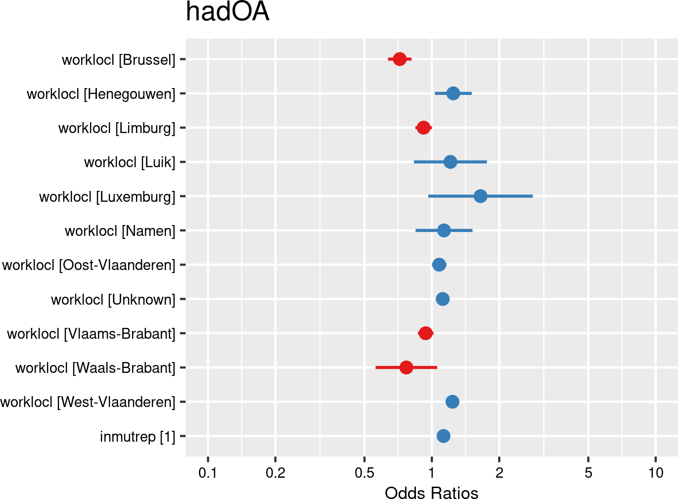

Work location categories (provinces) were introduced as fixed effects, and companies and employees as random effects. The model is based on data from employees with and without OAs from all mutual Liantis ESPP and PS customers. The model is adjusted for representativeness of the company (fixed effect inmutrep) regarding to sector, size and Flemish province.
According to Figure 3.134 (a) and Figure 3.134 (b), the province in which a worker works does not significantly determine the likelihood of a reported OA being rejected by the insurer.
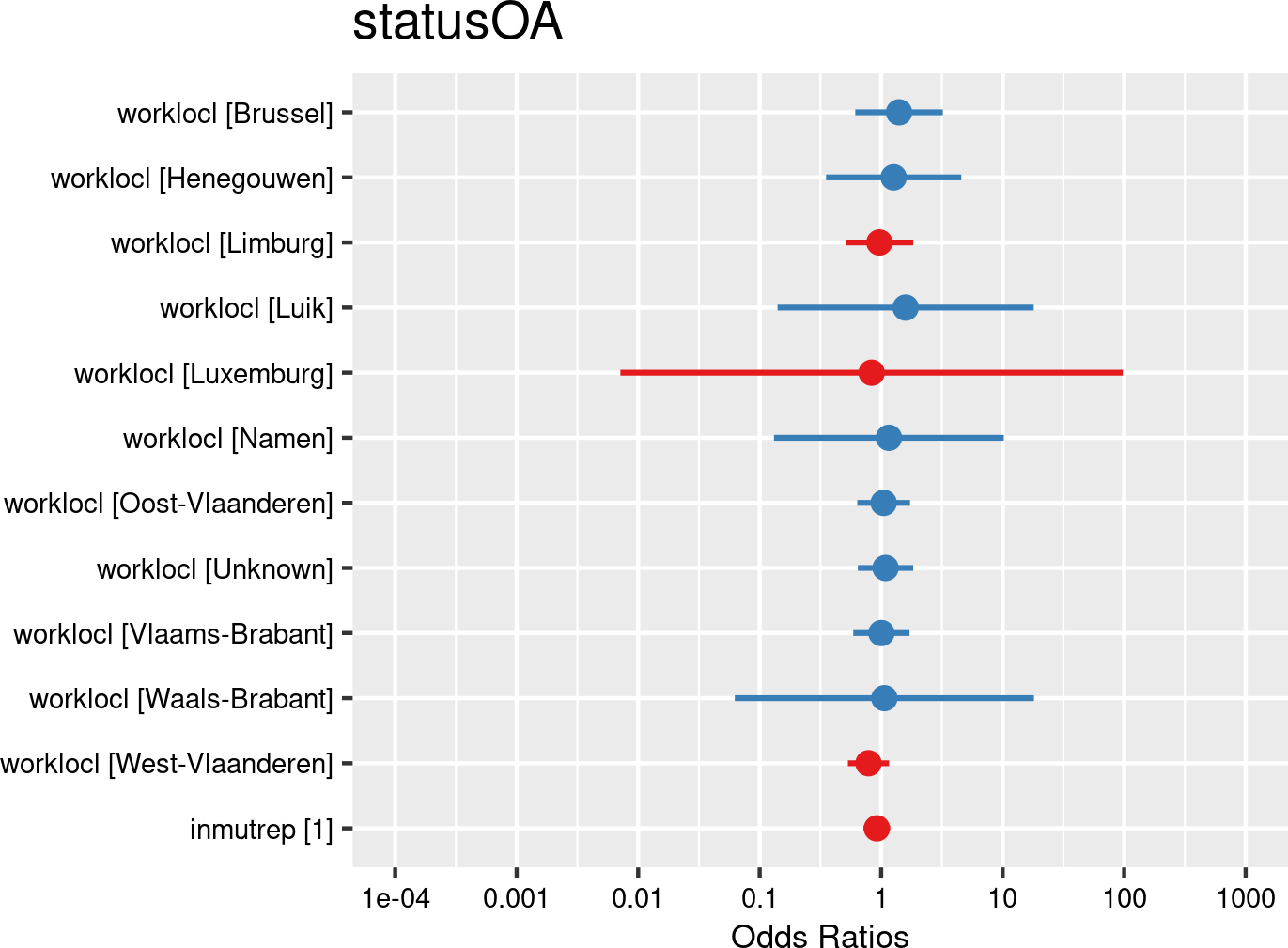

Work location categories (provinces) were introduced as fixed effects, and companies and employees as random effects. The model is based on data from employees notifying OAs from all mutual Liantis ESPP and PS customers. The model is adjusted for representativeness of the company (fixed effect inmutrep) regarding to sector, size and Flemish province.
According to Figure 3.135 (a) and Figure 3.135 (b), working in West Flanders significantly elevates the likelihood to have an accepted commuting accident.
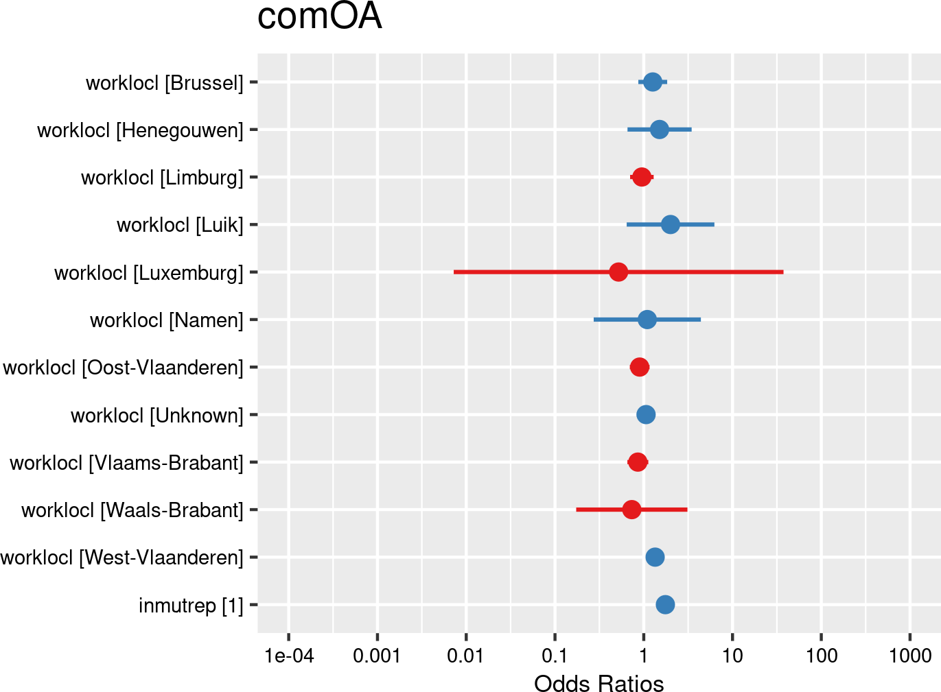

Work location categories (provinces) were introduced as fixed effects, and companies and employees as random effects. The model is based on data from employees with and without OAs from all mutual Liantis ESPP and PS customers. The model is adjusted for representativeness of the company (fixed effect inmutrep) regarding to sector, size and Flemish province.
Figure 3.136 (a) and Figure 3.136 (b) show that working in West Flanders, Luxembourg and Hainaut significantly increases the likelihood to have an accepted workplace accident, while working in Brussels decreases it. The lower odds for Brussels found in the present study is not in line with Federal Agency for Occupational Risks (2023) and might partially be explained by a higher proportion of white-collar workers in a smaller proportion of Liantis customers in this Region.
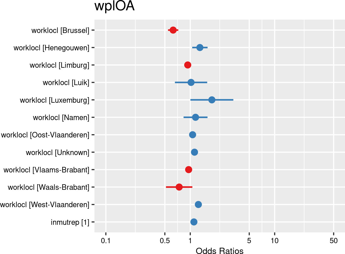

Work location categories (provinces) were introduced as fixed effects, and companies and employees as random effects. The model is based on data from employees with and without OAs from all mutual Liantis ESPP and PS customers. The model is adjusted for representativeness of the company (fixed effect inmutrep) regarding to sector, size and Flemish province.
Figure 3.137 (a) and Figure 3.137 (b) present a model estimating the frequency degree of OAs at the company level, contrasting with previous models that focused on individual employee accident probabilities. These figures show that a higher proportion of workers working in West-Flanders and Hainaut significantly increases the frequency degree of OAs within a company. On the contrary, a higher proportion workers from Limbourg and Brussels, significantly decreases the frequency degree of a company.
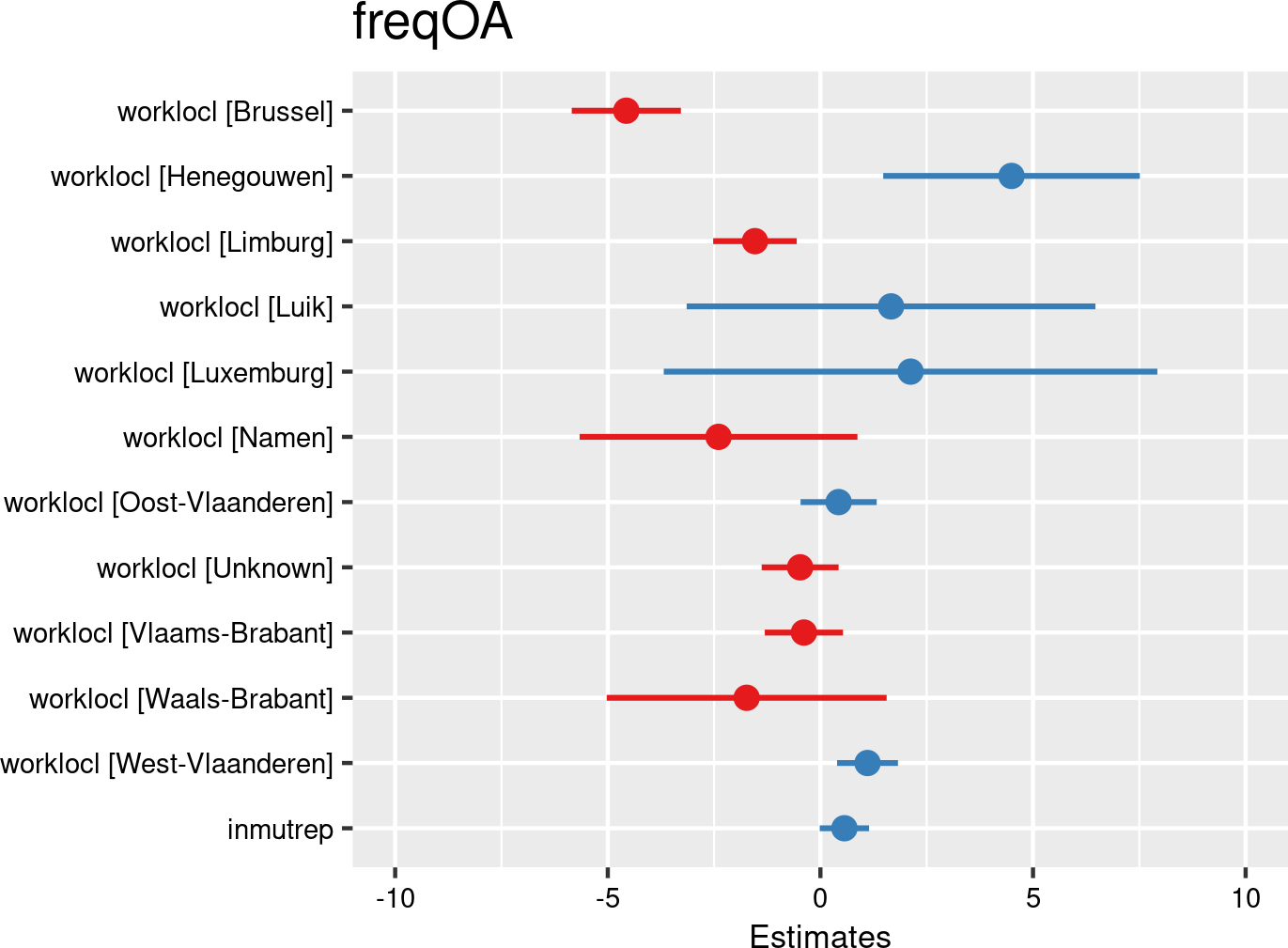

Work location categories (provinces) proportions were introduced as fixed effects, and companies as random effects. The model is based on data of all mutual Liantis ESPP and PS customers. The model is adjusted for representativeness of the company (fixed effect inmutrep) regarding to sector, size and Flemish province.
Figure 3.138 (a) and Figure 3.138 (b) present a model estimating the likelihood of an accepted accident being classified as serious according to Belgian law. These figures indicate that the province an employee is working in does not significantly determine the likelihood an OA is classified as serious.
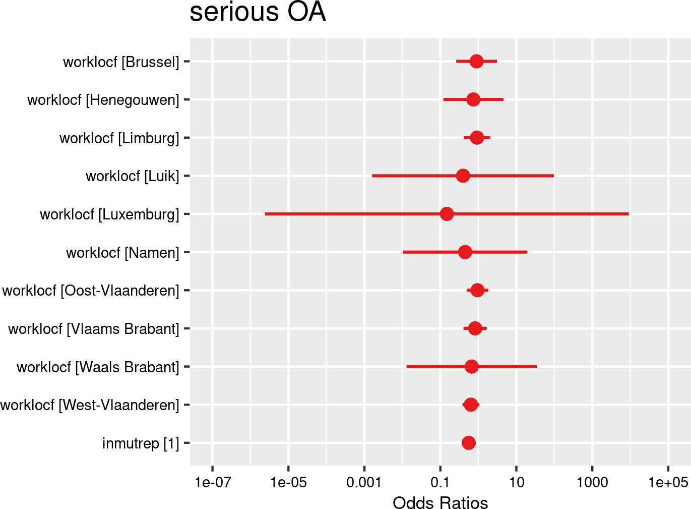

Work location categories (provinces) were introduced as fixed effects, and companies and employees as random effects. The model is based on data of all mutual Liantis ESPP and PS customers. The model is adjusted for representativeness of the company (fixed effect inmutrep) regarding to sector, size and Flemish province.
Figure 3.139 (a) and Figure 3.139 (b) show the results of a model assessing the relationship between work location and the number of absenteeism days. These figures are based on absenteeism data from FEDRIS, while Figure 3.140 (a) and Figure 3.140 (b) present the same model using data from Liantis PS. The figures indicate that workers who are working in Brussels and Flemish Brabant have a higher validated number of absenteeism days due to OAs (but not in West-Flanders). The number of validated accepted days off increases significantly for workers in Brussels, Flemish Brabant and Limbourg, with respectively 50% and 13% (but decreases in West-Flanders with 9%) in comparison with employees working in Antwerp.
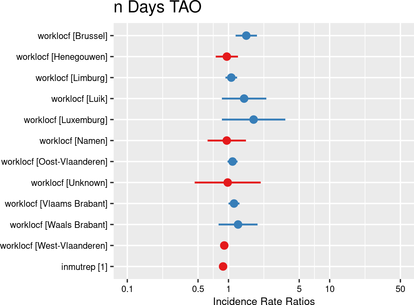

Work location categories (provinces) were introduced as fixed effects, and companies and employees as random effects. The model is based on data of all mutual Liantis ESPP and PS customers. The model is adjusted for representativeness of the company (fixed effect inmutrep) regarding to sector, size and Flemish province.
The model using Liantis PS calculated days partially confirms the previous model and shows a 34% increase in days off for working in Brussels.
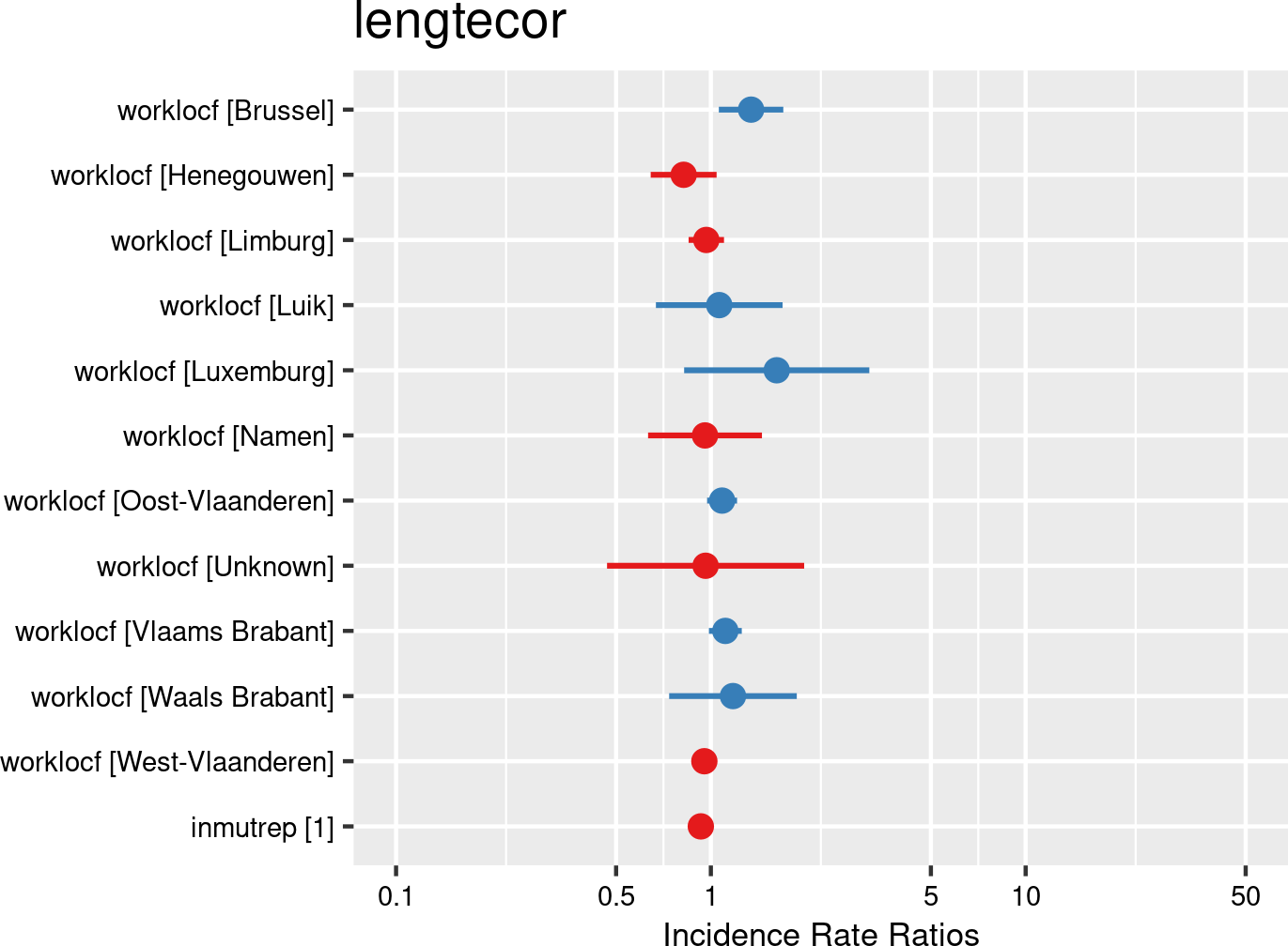

Work location categories (provinces) were introduced as fixed effects, and companies and employees as random effects. The model is based on data of all mutual Liantis ESPP and PS customers. The model is adjusted for representativeness of the company (fixed effect inmutrep) regarding to sector, size and Flemish province.
Figure 3.141 (a) and Figure 3.141 (b) show the results of a model evaluating the relationship between work location and the direct wage cost of an OA. The findings indicate some significant differences in direct wage cost related to an OA by the province an employer is located: for Limburg and West Flanders a significant lower result is found.
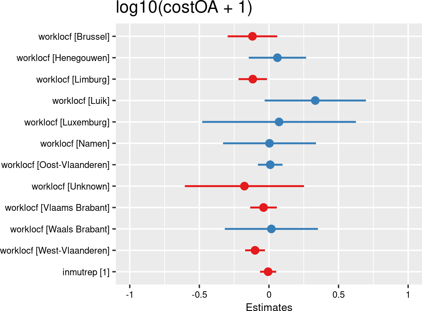

Work location categories (provinces) were introduced as fixed effects, and companies and employees as random effects. The model is based on data of all mutual Liantis ESPP and PS customers. The model is adjusted for representativeness of the company (fixed effect inmutrep) regarding to sector, size and Flemish province.
The next 4 figures (Figure 3.142 (a) and Figure 3.142 (b), Figure 3.143 (a) and Figure 3.143 (b)) are displaying the results of a model assessing the relation between proportion of workers living within a province and the severity degree of a company, which is again a variable at the company level. In the first model (Figure 3.142 (a) and Figure 3.142 (b)), validated number of absenteeism days from FEDRIS were used, while the second model Figure 3.143 (a) and Figure 3.143 (b)) was based on the numbers of days off in the Liantis PS data. The results of both models do not show an impact of the proportion of workers working in certain province on the severity degree of an employer.
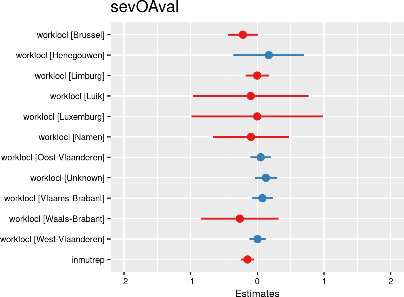

Work location categories (provinces) proportions were introduced as fixed effects, and companies as random effects. The model is based on data of all mutual Liantis ESPP and PS customers. The model is adjusted for representativeness of the company (fixed effect inmutrep) regarding to sector, size and Flemish province.
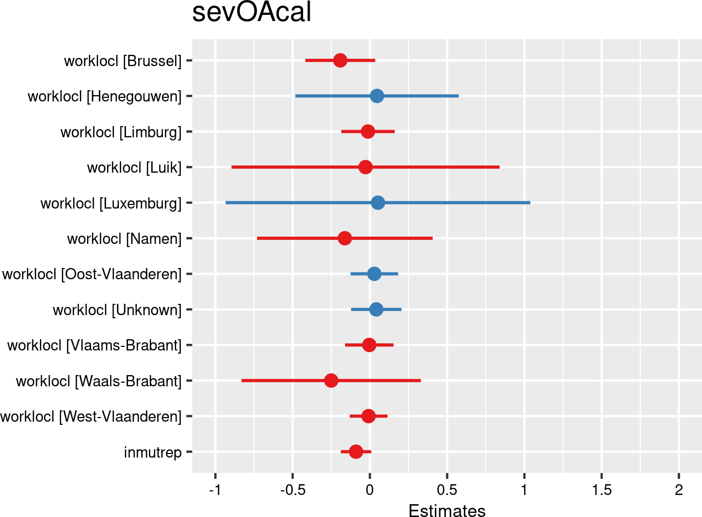

Work location categories (provinces) proportions were introduced as fixed effects, and companies as random effects. The model is based on data of all mutual Liantis ESPP and PS customers. The model is adjusted for representativeness of the company (fixed effect inmutrep) regarding to sector, size and Flemish province.
3.4.3.2 Company size
3.4.3.2.1 Descriptives
Both NSSO and FEDRIS provide statistics on size of the company. From Liantis PS data it is also possible to derive the size of the company through the number of employees. The notification in many cases also contains the size category of the employer. Since this information is also present in the notification information passed through to Liantis, the fit between the derived size of the employer of an employee experiencing an OA can be compared with the corresponding size classification in the original notification of the accident.
From Figure 3.144 we learn that the size derived from Liantis PS data and FEDRIS data are highly comparable when both are available. The correlation between the two datasets is >77%. This suggests that the size derived from Liantis PS data align well with those in FEDRIS data, making them suitable for further analysis.
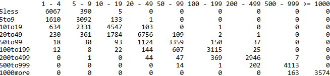
all accepted occupational accidents
| catsizef | rszall | rszpriv | liaall | fedrisall | totalnot | totalnotmut | totalnotrepmutflan |
|---|---|---|---|---|---|---|---|
| 1-4 werknemers | 7802224 | 7713792 | 3928642 | 79600 | 14015 | 10020 | 1973 |
| 5-9 werknemers | 6645987 | 6568088 | 2277552 | 68291 | 12397 | 7594 | 1517 |
| 10-19 werknemers | 8167741 | 8054595 | 3191538 | 93495 | 16278 | 8428 | 1885 |
| 20-49 werknemers | 12750195 | 12436450 | 3421511 | 161909 | 28428 | 10819 | 3360 |
| 50-99 werknemers | 9191192 | 8338008 | 1435969 | 121021 | 21174 | 6032 | 3578 |
| 100-199 werknemers | 10164557 | 8593060 | 1219028 | 129500 | 23599 | 5382 | 3533 |
| 200-499 werknemers | 13610892 | 11198182 | 1060267 | 164524 | 29712 | 4508 | 2872 |
| 500-999 werknemers | 9821180 | 8117406 | 879660 | 115253 | 18818 | 5095 | 3966 |
| ≥ 1000 werknemers | 47931892 | 23257774 | 641699 | 404541 | 30714 | 3338 | 3338 |
| Onbekend | NA | NA | NA | 15243 | 84 | 19 | 8 |
| catsizef | percrszall | percrszpriv | percliaall | percfedrisall | perctotalnot | perctotalnotmut | perctotalnotrepmutflan |
|---|---|---|---|---|---|---|---|
| 1-4 werknemers | 6.2 | 8.2 | 21.8 | 5.9 | 7.2 | 16.4 | 7.6 |
| 5-9 werknemers | 5.3 | 7.0 | 12.6 | 5.1 | 6.4 | 12.4 | 5.8 |
| 10-19 werknemers | 6.5 | 8.5 | 17.7 | 7.0 | 8.3 | 13.8 | 7.2 |
| 20-49 werknemers | 10.1 | 13.2 | 18.9 | 12.1 | 14.6 | 17.7 | 12.9 |
| 50-99 werknemers | 7.3 | 8.8 | 8.0 | 9.0 | 10.9 | 9.9 | 13.7 |
| 100-199 werknemers | 8.1 | 9.1 | 6.8 | 9.7 | 12.1 | 8.8 | 13.6 |
| 200-499 werknemers | 10.8 | 11.9 | 5.9 | 12.3 | 15.2 | 7.4 | 11.0 |
| 500-999 werknemers | 7.8 | 8.6 | 4.9 | 8.6 | 9.6 | 8.3 | 15.2 |
| ≥ 1000 werknemers | 38.0 | 24.7 | 3.6 | 30.2 | 15.7 | 5.5 | 12.8 |
| Onbekend | NA | NA | NA | NA | NA | NA | NA |
commuting accepted occupational accidents
| catsizef | rszall | rszpriv | liaall | fedrisall | totalnot | totalnotmut | totalnotrepmutflan |
|---|---|---|---|---|---|---|---|
| 1 - 4 werknemers | 7802224 | 7713792 | 3928642 | 10480 | 1629 | 1202 | 259 |
| 5 - 9 werknemers | 6645987 | 6568088 | 2277552 | 8708 | 1315 | 860 | 160 |
| 10 - 19 werknemers | 8167741 | 8054595 | 3191538 | 11837 | 1673 | 970 | 273 |
| 20 - 49 werknemers | 12750195 | 12436450 | 3421511 | 21823 | 3099 | 1285 | 430 |
| 50 - 99 werknemers | 9191192 | 8338008 | 1435969 | 18213 | 2712 | 959 | 541 |
| 100 - 199 werknemers | 10164557 | 8593060 | 1219028 | 21010 | 3477 | 998 | 706 |
| 200 - 499 werknemers | 13610892 | 11198182 | 1060267 | 29600 | 4807 | 863 | 524 |
| 500 - 999 werknemers | 9821180 | 8117406 | 879660 | 23039 | 3244 | 957 | 715 |
| ≥ 1000 werknemers | 47931892 | 23257774 | 641699 | 79522 | 6420 | 502 | 502 |
| Onbekend | NA | NA | NA | 2078 | 11 | 3 | 2 |
| catsizef | percrszall | percrszpriv | percliaall | percfedrisall | perctotalnot | perctotalnotmut | perctotalnotrepmutflan |
|---|---|---|---|---|---|---|---|
| 1 - 4 werknemers | 6.2 | 8.2 | 21.8 | 4.7 | 5.7 | 14.0 | 6.3 |
| 5 - 9 werknemers | 5.3 | 7.0 | 12.6 | 3.9 | 4.6 | 10.0 | 3.9 |
| 10 - 19 werknemers | 6.5 | 8.5 | 17.7 | 5.3 | 5.9 | 11.3 | 6.6 |
| 20 - 49 werknemers | 10.1 | 13.2 | 18.9 | 9.7 | 10.9 | 14.9 | 10.5 |
| 50 - 99 werknemers | 7.3 | 8.8 | 8.0 | 8.1 | 9.6 | 11.2 | 13.2 |
| 100 - 199 werknemers | 8.1 | 9.1 | 6.8 | 9.4 | 12.3 | 11.6 | 17.2 |
| 200 - 499 werknemers | 10.8 | 11.9 | 5.9 | 13.2 | 16.9 | 10.0 | 12.7 |
| 500 - 999 werknemers | 7.8 | 8.6 | 4.9 | 10.3 | 11.4 | 11.1 | 17.4 |
| ≥ 1000 werknemers | 38.0 | 24.7 | 3.6 | 35.5 | 22.6 | 5.8 | 12.2 |
| Onbekend | NA | NA | NA | NA | NA | NA | NA |
workplace accepted occupational accidents
| catsizef | rszall | rszpriv | liaall | fedrisall | totalnot | totalnotmut | totalnotrepmutflan |
|---|---|---|---|---|---|---|---|
| 1-4 werknemers | 7802224 | 7713792 | 3928642 | 69120 | 12386 | 8818 | 1714 |
| 5-9 werknemers | 6645987 | 6568088 | 2277552 | 59583 | 11082 | 6734 | 1357 |
| 10-19 werknemers | 8167741 | 8054595 | 3191538 | 81658 | 14605 | 7458 | 1612 |
| 20-49 werknemers | 12750195 | 12436450 | 3421511 | 140086 | 25329 | 9534 | 2930 |
| 50-99 werknemers | 9191192 | 8338008 | 1435969 | 102808 | 18462 | 5073 | 3037 |
| 100-199 werknemers | 10164557 | 8593060 | 1219028 | 108490 | 20122 | 4384 | 2827 |
| 200-499 werknemers | 13610892 | 11198182 | 1060267 | 134924 | 24905 | 3645 | 2348 |
| 500-999 werknemers | 9821180 | 8117406 | 879660 | 92214 | 15574 | 4138 | 3251 |
| ≥ 1000 werknemers | 47931892 | 23257774 | 641699 | 325019 | 24294 | 2836 | 2836 |
| Onbekend | NA | NA | NA | 13165 | 73 | 16 | 6 |
| catsizef | percrszall | percrszpriv | percliaall | percfedrisall | perctotalnot | perctotalnotmut | perctotalnotrepmutflan |
|---|---|---|---|---|---|---|---|
| 1-4 werknemers | 6.2 | 8.2 | 21.8 | 6.2 | 7.4 | 16.8 | 7.8 |
| 5-9 werknemers | 5.3 | 7.0 | 12.6 | 5.3 | 6.6 | 12.8 | 6.2 |
| 10-19 werknemers | 6.5 | 8.5 | 17.7 | 7.3 | 8.8 | 14.2 | 7.4 |
| 20-49 werknemers | 10.1 | 13.2 | 18.9 | 12.6 | 15.2 | 18.1 | 13.4 |
| 50-99 werknemers | 7.3 | 8.8 | 8.0 | 9.2 | 11.1 | 9.6 | 13.9 |
| 100-199 werknemers | 8.1 | 9.1 | 6.8 | 9.7 | 12.1 | 8.3 | 12.9 |
| 200-499 werknemers | 10.8 | 11.9 | 5.9 | 12.1 | 14.9 | 6.9 | 10.7 |
| 500-999 werknemers | 7.8 | 8.6 | 4.9 | 8.3 | 9.3 | 7.9 | 14.8 |
| ≥ 1000 werknemers | 38.0 | 24.7 | 3.6 | 29.2 | 14.6 | 5.4 | 12.9 |
| Onbekend | NA | NA | NA | NA | NA | NA | NA |
3.4.3.2.2 Models
The following Table 3.98 table summarizes the results of the models assessing the relationship between company size categories and the several outcomes related to OAs. Below the table, details are provided about the data used for the analyses. The results of the nine models are then presented both graphically and in a table.
| catsize | chance to notify | chance on refusal | chance commuting | chance workplace | freq degree | chance serious | nDays TAO V/C | cost | sev degree V/C |
|---|---|---|---|---|---|---|---|---|---|
| < 5 | REF | REF | REF | REF | ns | REF | REF | REF | ns |
| 5 to 9 | > | ns | > | > | > | ns | ns/ns | ns | ns |
| 10 to 19 | > | ns | > | > | > | ns | </< | ns | ns |
| 20 to 49 | > | ns | > | > | > | ns | </< | < | ns |
| 50 to 99 | > | ns | > | > | > | < | </< | < | ns |
| 100 to 199 | > | > | > | > | > | < | </< | ns | ns |
| 200 to 499 | > | ns | > | > | > | < | </< | ns | ns |
| 500 to 999 | > | ns | > | > | > | < | </ns | < | ns |
| >= 1000 | > | ns | > | ns | ns | < | </< | < | ns |
| occur | accept | occur | occur | occur | severe | severe | severe | severe | |
| empl | empl | empl | empl | comp | empl | empl | empl | comp | |
| c/w all | c/w ref | c acc | w acc | w acc | w acc | w acc | w acc | w acc |
- occur: data include all workers, chance for occurrence is calculated for the outcome
- accept: data include only workers with a notification of OA
- severe: data include only workers with an accepted OA
- c/w all: commuting and workplace accidents, including refused and accidents without decisions
- c/w ref: accepted or refused commuting and workplace accidents
- c acc: accepted commuting accidents
- w acc: accepted workplace accidents
- empl: the outcome is situated at the individual level
- comp: the outcome is situated at the company level
- nDaysTAO: number of days absenteeism related to the OA
- V/C: Validated number of days (available from FEDRIS) / Calculated number of days (based on the Liantis PS data)
Company size and occupational accidents
- The likelihood for an accepted commuting accident gradually and significantly increases with company size. The overall likelihood to report an occupational accident and the likelihood for an accepted workplace accident increases for companies up up to 199 workers and then decreases again (with wider confidence intervals).
- Except for companies in the category of 100 to 199 workers, size of the company does not seem to determine the chance on refusal of an occupational accident by the insurer.
- Company size significantly determines whether an workplace occupational accident is classified as serious: the larger the company, the lower the likelihood.
- The number of absence days associated with an accepted workplace accidents significantly decreases with company size, as well as the direct wage cost for the employer.
- At company level, company size does significantly determine the frequency degree of a company, but not the severity degree.
From Figure 3.145 (a) and Figure 3.145 (b) we learn that likelihood of notifying an OA varies substantially across employer size categories. Compared to the reference employer group (<5 employees), larger employers (up to 200 employees) generally show higher odds, the odds ratio increasing progressively with size. Beyond 200 employees, the odds ratios tend to stabilize and to show wider confidence intervals, indicating variability and potential uncertainty in the estimates.
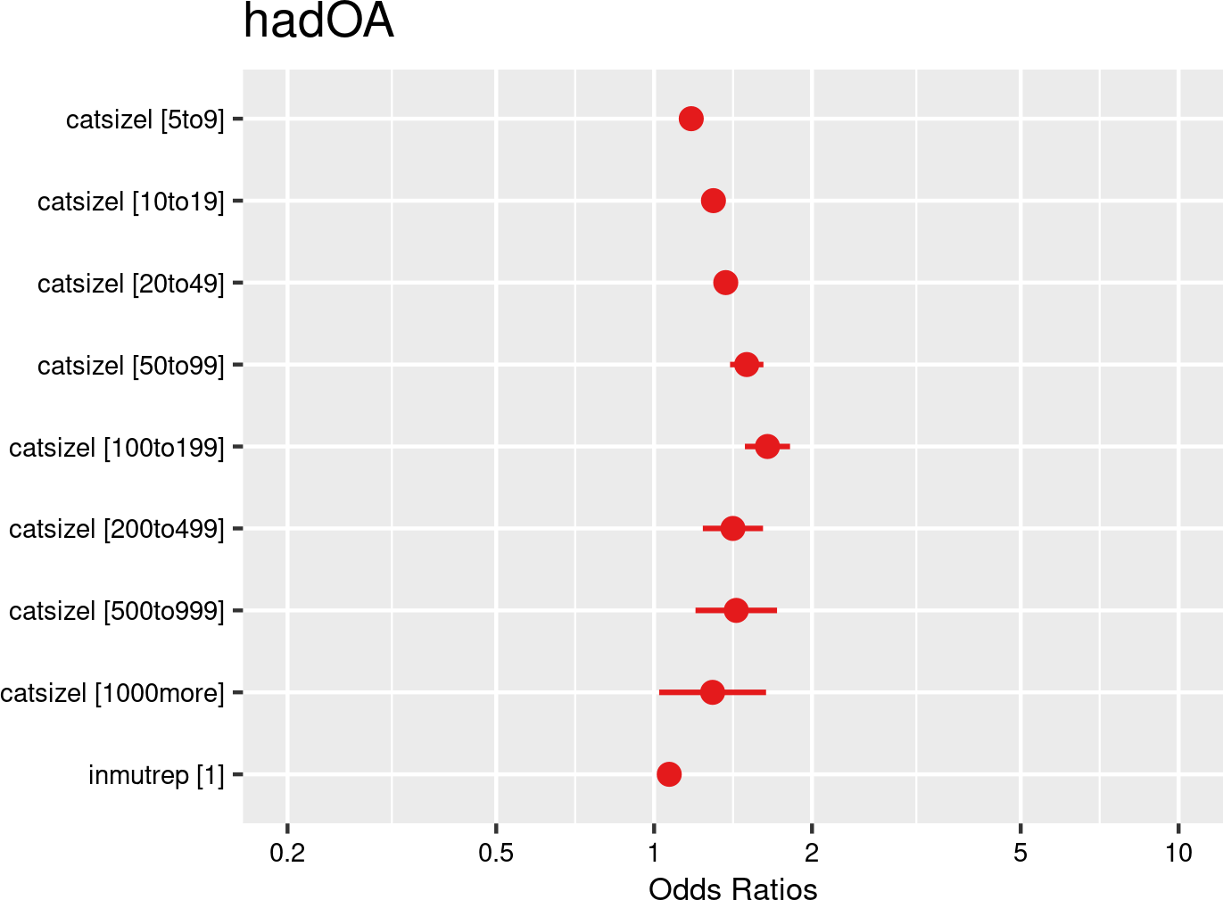

Company size categories were introduced as fixed effects, and companies and employees as random effects. The model is based on data from employees with and without OAs from all mutual Liantis ESPP and PS customers. The model is adjusted for representativeness of the company (fixed effect inmutrep) regarding to sector, size and Flemish province.
According to Figure 3.146 (a) and Figure 3.146 (b), companies with 100 to 199 employees have a significantly higher likelihood of having an OA refused by the insurer compared to companies with fewer than 5 employees (the reference category). For other company size categories, the odds ratios do not show any significant differences.
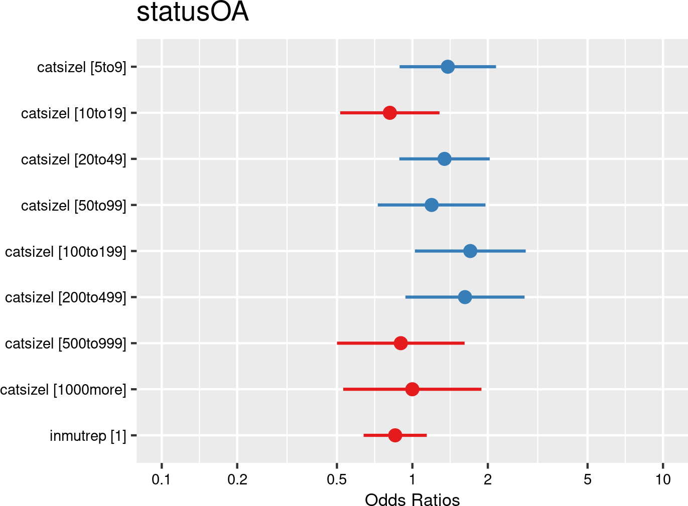

Company size categories were introduced as fixed effects, and companies and employees as random effects. The model is based on data from employees notifying OAs from all mutual Liantis ESPP and PS customers. The model is adjusted for representativeness of the company (fixed effect inmutrep) regarding to sector, size and Flemish province.
According to Figure 3.147 (a) and Figure 3.147 (b), working within larger employers implicates a higher likelihood for employees experiencing accepted commuting accidents.
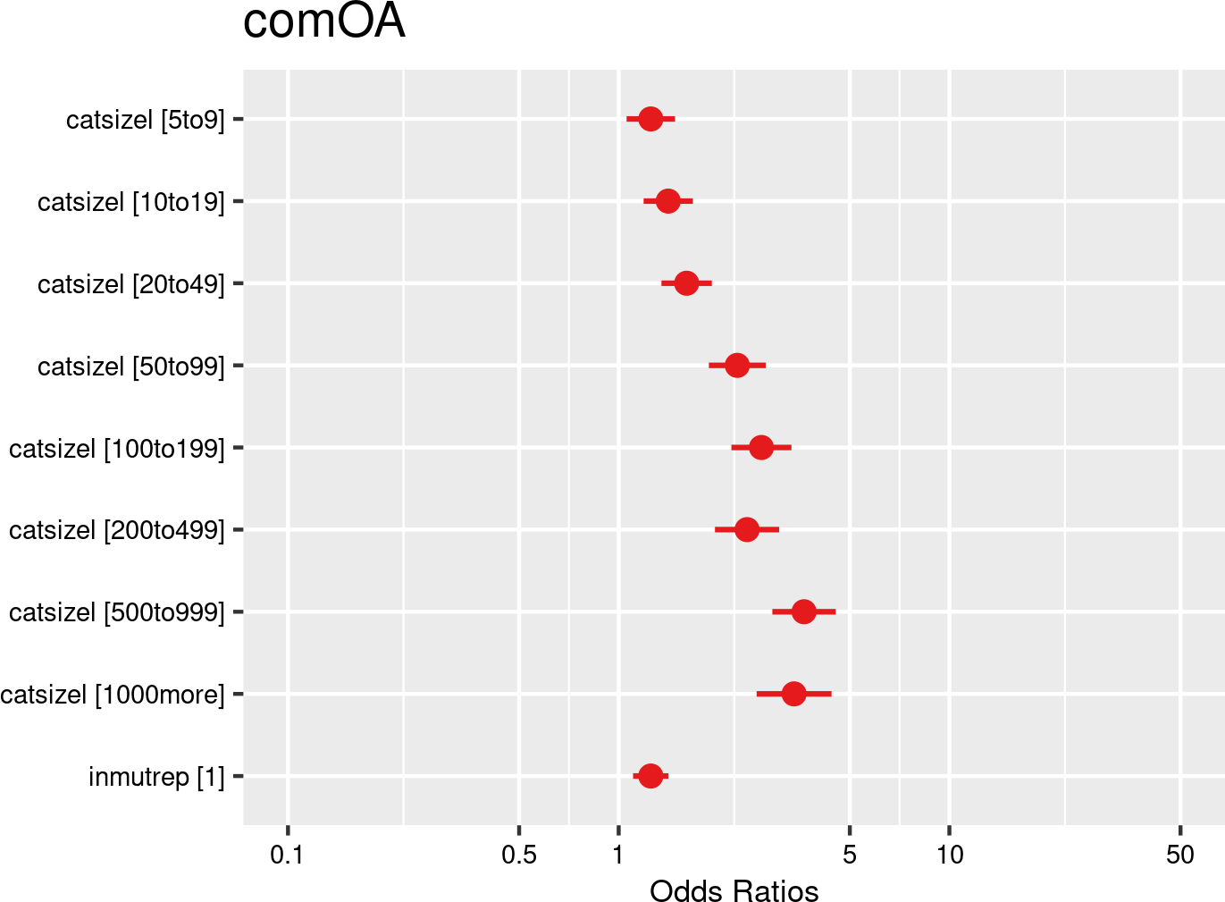

Company size categories were introduced as fixed effects, and companies and employees as random effects. The model is based on data from employees with and without OAs from all mutual Liantis ESPP and PS customers. The model is adjusted for representativeness of the company (fixed effect inmutrep) regarding to sector, size and Flemish province.
Figure 3.148 (a) and Figure 3.148 (b) show that for employers up to 200 employees, the odds ratios for accepted workplace accidents increase with company size. For larger companies, odds ratios decrease again, although the confidence intervals are wider. For companies with 1000 or more employees, the odds ratio is not significantly different from the reference category.
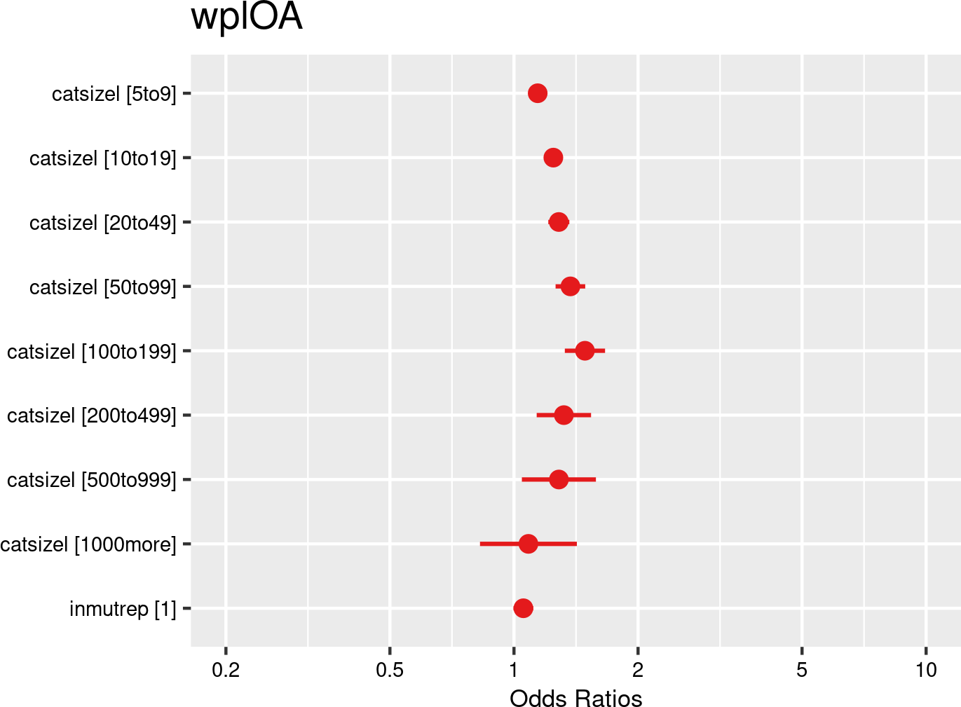

Company size categories were introduced as fixed effects, and companies and employees as random effects. The model is based on data from employees with and without OAs from all mutual Liantis ESPP and PS customers. The model is adjusted for representativeness of the company (fixed effect inmutrep) regarding to sector, size and Flemish province.
Figure 3.149 (a) and Figure 3.149 (b) present a model estimating the frequency degree of OAs at the company level, in contrast to previous models that focused on individual employee accident probabilities. These figures show that a larger company size corresponds to a higher frequency degree within a company.
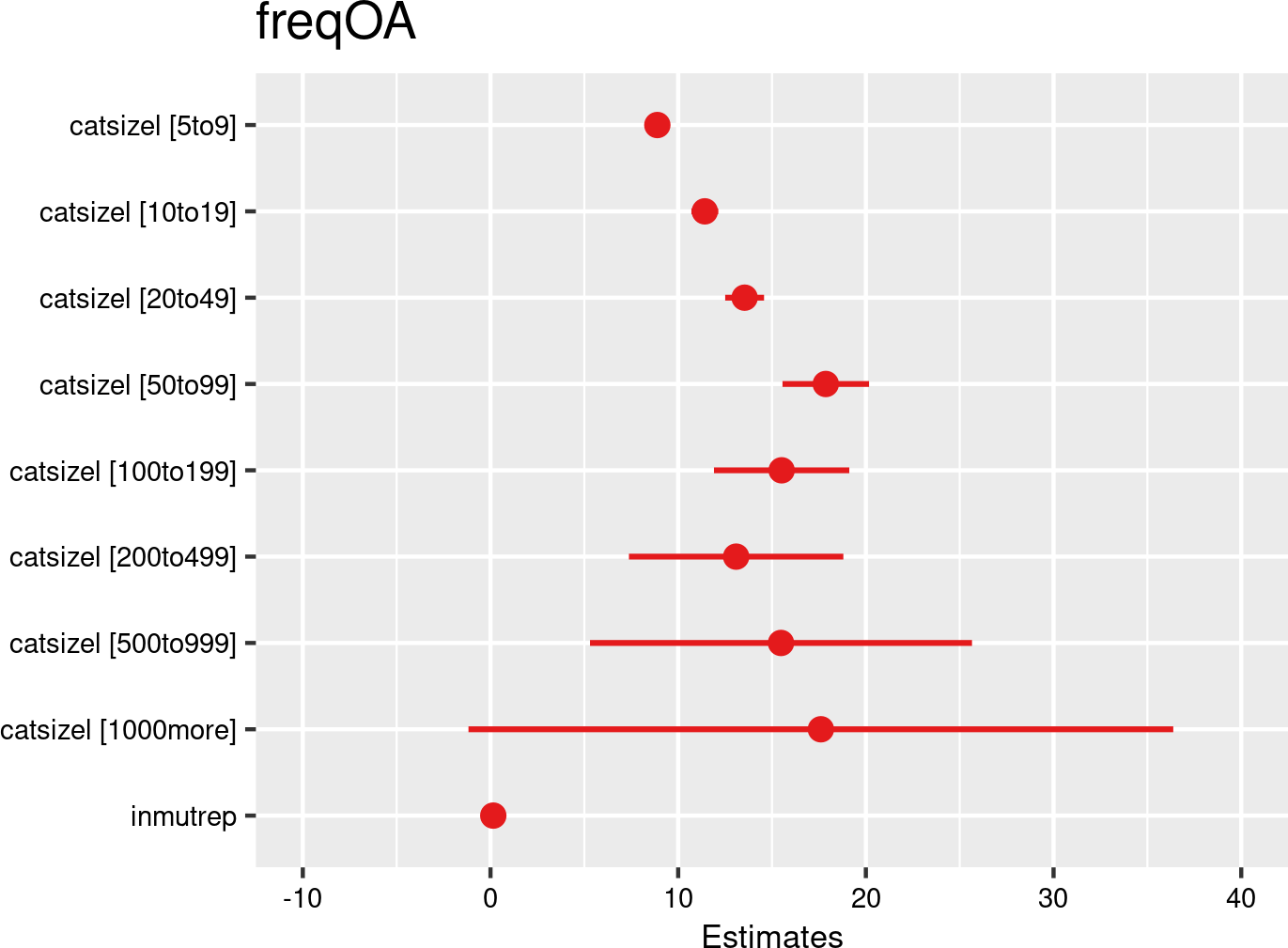

Company size categories proportions were introduced as fixed effects, and companies as random effects. The model is based on data of all mutual Liantis ESPP and PS customers. The model is adjusted for representativeness of the company (fixed effect inmutrep) regarding to sector, size and Flemish province.
Figure 3.150 (a) and Figure 3.150 (b) present a model estimating the chance for an accepted accident being serious (according to the definition of the Belgian law). These figures indicate that company size does significantly determine whether an workplace OA is classified as serious: the larger the company, the lower the odds.
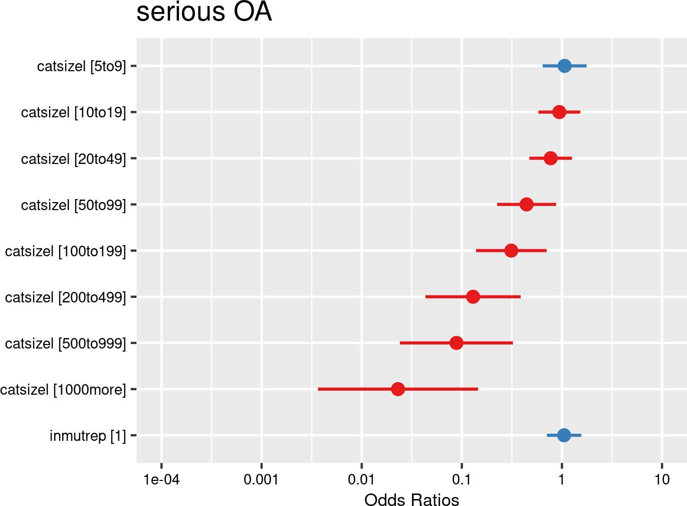

Company size categories were introduced as fixed effects, and companies and employees as random effects. The model is based on data of all mutual Liantis ESPP and PS customers. The model is adjusted for representativeness of the company (fixed effect inmutrep) regarding to sector, size and Flemish province.
Figure 3.151 (a) and Figure 3.151 (b) and Figure 3.152 (a) and Figure 3.152 (b) do not confirm previous literature (Fabiano et al., 2004; Kines & Mikkelsen, 2003; McVittie et al., 1997) that smaller companies report a lower number of days absent from work due to an accepted workplace accidents. The trend in our results is rather that number of days decreases when company sizes get larger.
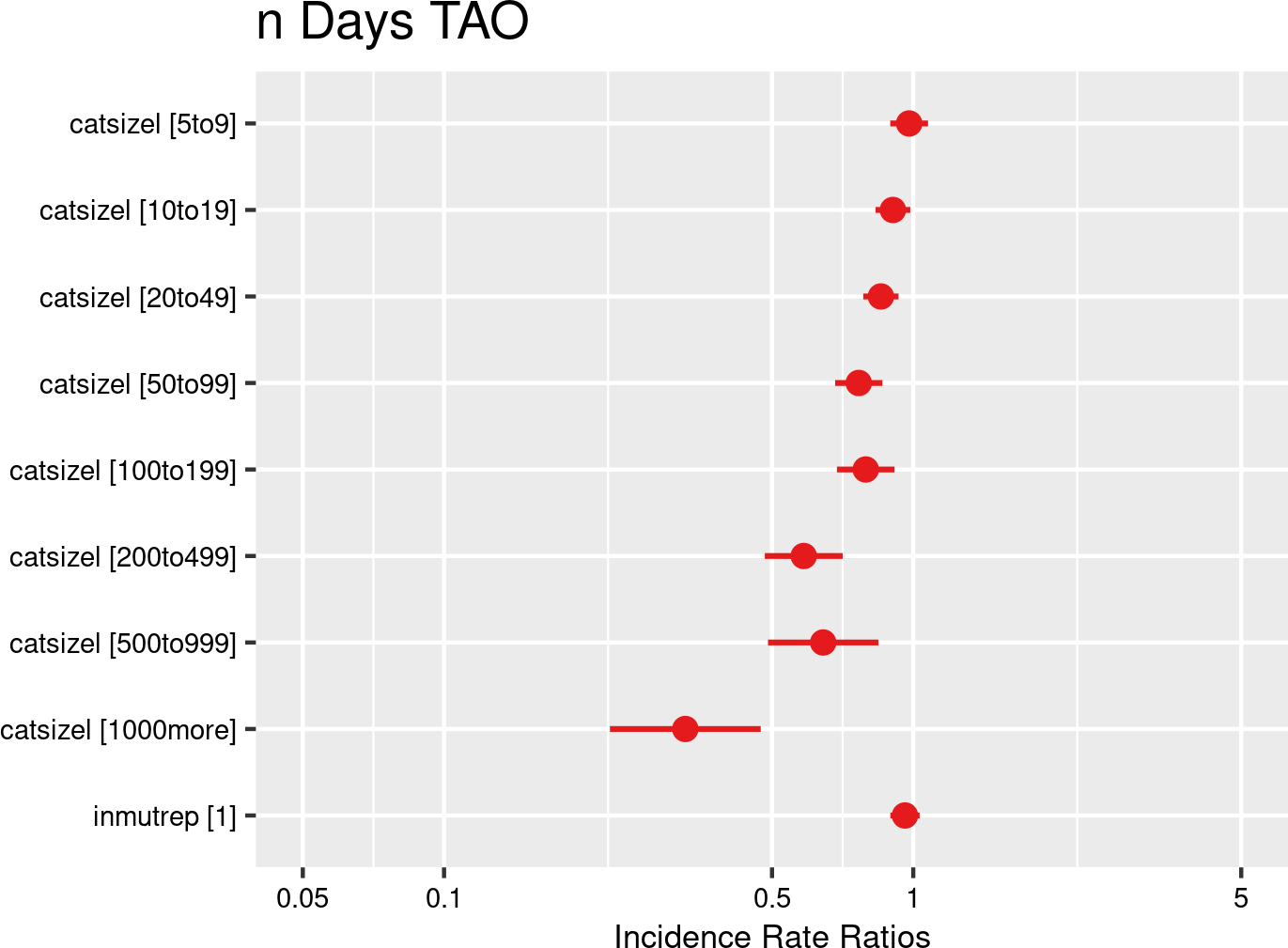

Company size categories were introduced as fixed effects, and companies and employees as random effects. The model is based on data of all mutual Liantis ESPP and PS customers. The model is adjusted for representativeness of the company (fixed effect inmutrep) regarding to sector, size and Flemish province.
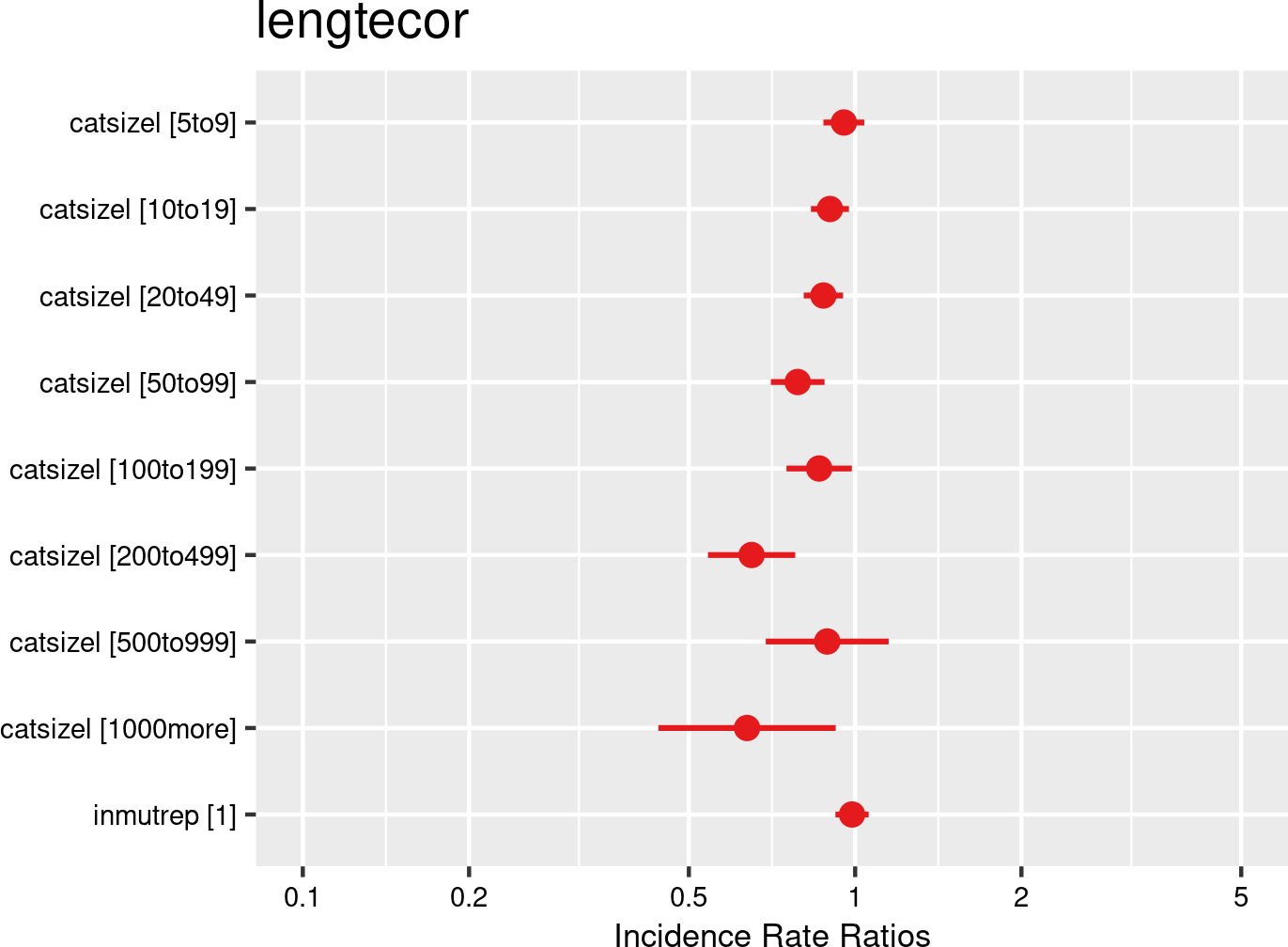

Company size categories were introduced as fixed effects, and companies and employees as random effects. The model is based on data of all mutual Liantis ESPP and PS customers. The model is adjusted for representativeness of the company (fixed effect inmutrep) regarding to sector, size and Flemish province.
Figure 3.153 (a) and Figure 3.153 (b) demonstrate that company size significantly influences the direct wage cost incurred by an employer following an accepted workplace accident. Among companies with 50 or more employees, a cler trend emerges: the larger the company, the lower the direct wage cost. However, the confidence intervals also widen as company size increases.
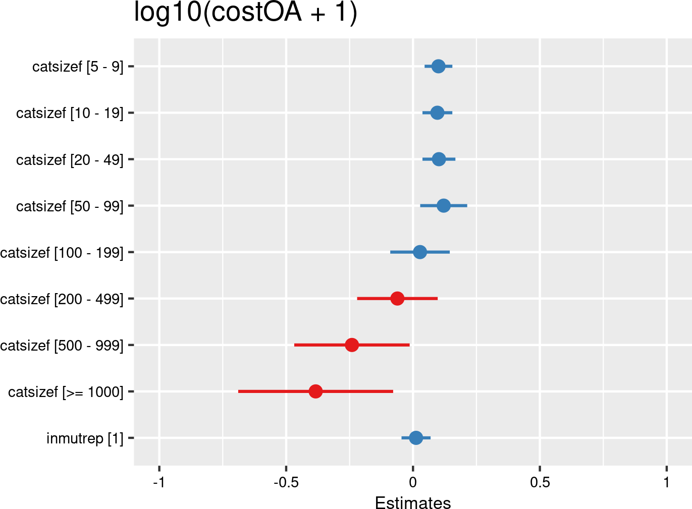

Company size categories were introduced as fixed effects, and companies and employees as random effects. The model is based on data of all mutual Liantis ESPP and PS customers. The model is adjusted for representativeness of the company (fixed effect inmutrep) regarding to sector, size and Flemish province.
The next 4 figures (Figure 3.154 (a) and Figure 3.154 (b), Figure 3.155 (a) and Figure 3.155 (b)) indicate that company size does not significantly determine the severity degree of a company.
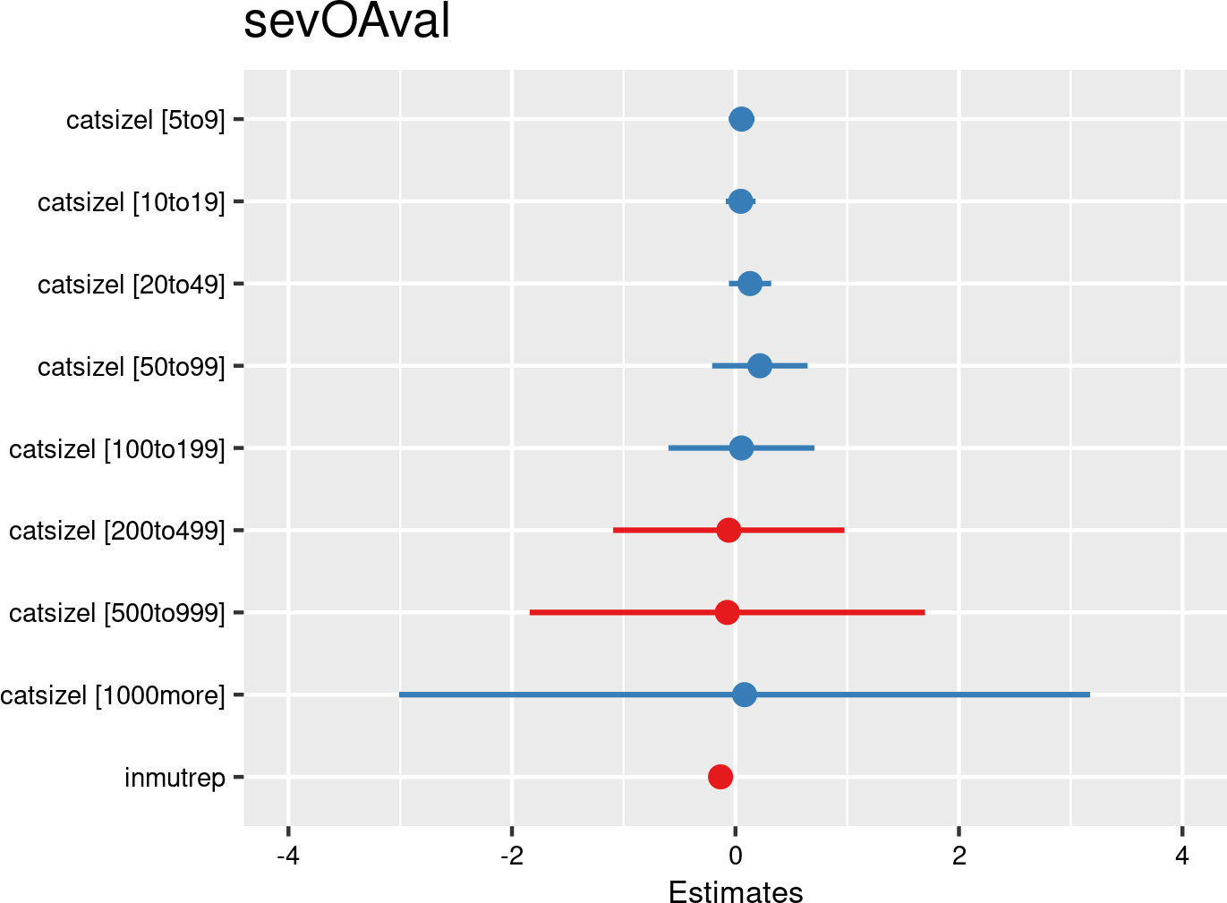

Company size categories proportions were introduced as fixed effects, and companies as random effects. The model is based on data of all mutual Liantis ESPP and PS customers. The model is adjusted for representativeness of the company (fixed effect inmutrep) regarding to sector, size and Flemish province.
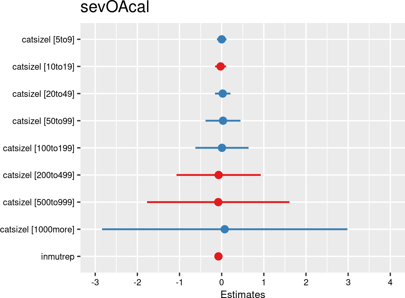

Company size categories proportions were introduced as fixed effects, and companies as random effects. The model is based on data of all mutual Liantis ESPP and PS customers. The model is adjusted for representativeness of the company (fixed effect inmutrep) regarding to sector, size and Flemish province.
3.4.3.3 Precarious employment
3.4.3.3.1 Subcontracting
Data Quality Alert: subcontracting
- Liantis (neither ESPP nor PS) does not have information on the frequencies with which all employees are exposed to work activities as subcontractors like FEDRIS describes in the context of occupational accidents
- Information on subcontracting would only be present in occupational accident notifications received via FEDRIS but almost no positive validations are detected (see Section 2.7.2.4)
Within Liantis, no systematically maintained variables related to subcontracting are currently available that would allow for investigation of a potential association with occupational accidents. As a result, no further analyses or modelling efforts were undertaken in relation to subcontracting.
3.4.3.5 Insurance companies
3.4.3.5.1 Descriptives
Neither NSSO nor FEDRIS provide statistics on the insurer of the employee. However, each OA notification includes the legal insurer’s identification number. Through Liantis Risk Solutions (RS), it is possible to link annual insurer fee payments for Liantis customers.
To estimate the insurer for employees who did not experience an OA, we applied the following method: we grouped data by employer, sorted it chronologically, and propagated the most recently known insurer number forward until a new insurer number was identified. Either through an employee’s OA notification or through Liantis RS data.
If no Liantis RS data was available for an employer and no OA occurred during the study period, we were unable to infer the insurer. These cases were excluded from the analysis.
Data Quality Alert: insurance companies
- Liantis (neither via ESPP nor PS) has structurally available data on the occupational accident (OA) insurer for all its client employers, as described by FEDRIS in the context of occupational accidents.
- However, since insurer information is consistently included in OA notifications received via FEDRIS (see Section 2.7.3.9), and OA insurance is typically managed at the employer level rather than the employee level, it is often possible to infer the insurer for employees who did not experience an OA.
Currently, Liantis does not maintain any systematically structured variables related to the occupational accident insurer. Nevertheless, with minimal assumptions, it may be feasible to explore whether the insurer has an influence on the occurrence and severity of occupational accidents.
all accepted occupational accidents
| catnrins | rszall | rszpriv | liaall | fedrisall | totalnot | totalnotmut | totalnotrepmutflan |
|---|---|---|---|---|---|---|---|
| pseudins01 | NA | NA | NA | NA | 9715 | 4470 | 1601 |
| pseudins02 | NA | NA | NA | NA | 18340 | 9459 | 4455 |
| pseudins03 | NA | NA | NA | NA | 15804 | 4231 | 1900 |
| pseudins04 | NA | NA | NA | NA | 3951 | 1756 | 651 |
| pseudins05 | NA | NA | NA | NA | 18396 | 9881 | 3664 |
| pseudins06 | NA | NA | NA | NA | 28 | NA | NA |
| pseudins07 | NA | NA | NA | NA | 12799 | 2 | NA |
| pseudins08 | NA | NA | NA | NA | 35943 | 9209 | 3533 |
| pseudins09 | NA | NA | NA | NA | 7632 | 3138 | 1669 |
| pseudins10 | NA | NA | NA | NA | 7421 | 2383 | 750 |
| pseudins11 | NA | NA | NA | NA | 21080 | 5813 | 3581 |
| pseudins12 | NA | NA | NA | NA | 44086 | 10877 | 4226 |
| pseudins13 | NA | NA | NA | NA | 24 | 16 | NA |
| catnrins | percrszall | percrszpriv | percliaall | percfedrisall | perctotalnot | perctotalnotmut | perctotalnotrepmutflan |
|---|---|---|---|---|---|---|---|
| pseudins01 | NA | NA | NA | NA | 4.98 | 7.30 | 6.15 |
| pseudins02 | NA | NA | NA | NA | 9.39 | 15.45 | 17.11 |
| pseudins03 | NA | NA | NA | NA | 8.10 | 6.91 | 7.30 |
| pseudins04 | NA | NA | NA | NA | 2.02 | 2.87 | 2.50 |
| pseudins05 | NA | NA | NA | NA | 9.42 | 16.14 | 14.08 |
| pseudins06 | NA | NA | NA | NA | 0.01 | NA | NA |
| pseudins07 | NA | NA | NA | NA | 6.56 | 0.00 | NA |
| pseudins08 | NA | NA | NA | NA | 18.41 | 15.04 | 13.57 |
| pseudins09 | NA | NA | NA | NA | 3.91 | 5.12 | 6.41 |
| pseudins10 | NA | NA | NA | NA | 3.80 | 3.89 | 2.88 |
| pseudins11 | NA | NA | NA | NA | 10.80 | 9.49 | 13.76 |
| pseudins12 | NA | NA | NA | NA | 22.58 | 17.76 | 16.24 |
| pseudins13 | NA | NA | NA | NA | 0.01 | 0.03 | NA |
commuting accepted occupational accidents
| catnrins | rszall | rszpriv | liaall | fedrisall | totalnot | totalnotmut | totalnotrepmutflan |
|---|---|---|---|---|---|---|---|
| pseudins01 | NA | NA | NA | NA | 1470 | 698 | 337 |
| pseudins02 | NA | NA | NA | NA | 2942 | 1452 | 755 |
| pseudins03 | NA | NA | NA | NA | 2089 | 548 | 291 |
| pseudins04 | NA | NA | NA | NA | 526 | 215 | 89 |
| pseudins05 | NA | NA | NA | NA | 2512 | 1338 | 526 |
| pseudins07 | NA | NA | NA | NA | 2501 | 1 | NA |
| pseudins08 | NA | NA | NA | NA | 5708 | 1322 | 656 |
| pseudins09 | NA | NA | NA | NA | 468 | 243 | 170 |
| pseudins10 | NA | NA | NA | NA | 1291 | 409 | 114 |
| pseudins11 | NA | NA | NA | NA | 3225 | 1004 | 621 |
| pseudins12 | NA | NA | NA | NA | 5654 | 1368 | 553 |
| pseudins13 | NA | NA | NA | NA | 1 | 1 | NA |
| catnrins | percrszall | percrszpriv | percliaall | percfedrisall | perctotalnot | perctotalnotmut | perctotalnotrepmutflan |
|---|---|---|---|---|---|---|---|
| pseudins01 | NA | NA | NA | NA | 5.18 | 8.12 | 8.20 |
| pseudins02 | NA | NA | NA | NA | 10.36 | 16.89 | 18.36 |
| pseudins03 | NA | NA | NA | NA | 7.36 | 6.37 | 7.08 |
| pseudins04 | NA | NA | NA | NA | 1.85 | 2.50 | 2.16 |
| pseudins05 | NA | NA | NA | NA | 8.85 | 15.56 | 12.79 |
| pseudins07 | NA | NA | NA | NA | 8.81 | 0.01 | NA |
| pseudins08 | NA | NA | NA | NA | 20.11 | 15.37 | 15.95 |
| pseudins09 | NA | NA | NA | NA | 1.65 | 2.83 | 4.13 |
| pseudins10 | NA | NA | NA | NA | 4.55 | 4.76 | 2.77 |
| pseudins11 | NA | NA | NA | NA | 11.36 | 11.68 | 15.10 |
| pseudins12 | NA | NA | NA | NA | 19.92 | 15.91 | 13.45 |
| pseudins13 | NA | NA | NA | NA | 0.00 | 0.01 | NA |
workplace accepted occupational accidents
| catnrins | rszall | rszpriv | liaall | fedrisall | totalnot | totalnotmut | totalnotrepmutflan |
|---|---|---|---|---|---|---|---|
| pseudins01 | NA | NA | NA | NA | 8245 | 3772 | 1264 |
| pseudins02 | NA | NA | NA | NA | 15398 | 8007 | 3700 |
| pseudins03 | NA | NA | NA | NA | 13715 | 3683 | 1609 |
| pseudins04 | NA | NA | NA | NA | 3425 | 1541 | 562 |
| pseudins05 | NA | NA | NA | NA | 15884 | 8543 | 3138 |
| pseudins06 | NA | NA | NA | NA | 28 | NA | NA |
| pseudins07 | NA | NA | NA | NA | 10298 | 1 | NA |
| pseudins08 | NA | NA | NA | NA | 30235 | 7887 | 2877 |
| pseudins09 | NA | NA | NA | NA | 7164 | 2895 | 1499 |
| pseudins10 | NA | NA | NA | NA | 6130 | 1974 | 636 |
| pseudins11 | NA | NA | NA | NA | 17855 | 4809 | 2960 |
| pseudins12 | NA | NA | NA | NA | 38432 | 9509 | 3673 |
| pseudins13 | NA | NA | NA | NA | 23 | 15 | NA |
| catnrins | percrszall | percrszpriv | percliaall | percfedrisall | perctotalnot | perctotalnotmut | perctotalnotrepmutflan |
|---|---|---|---|---|---|---|---|
| pseudins01 | NA | NA | NA | NA | 4.94 | 7.17 | 5.77 |
| pseudins02 | NA | NA | NA | NA | 9.23 | 15.21 | 16.88 |
| pseudins03 | NA | NA | NA | NA | 8.22 | 7.00 | 7.34 |
| pseudins04 | NA | NA | NA | NA | 2.05 | 2.93 | 2.56 |
| pseudins05 | NA | NA | NA | NA | 9.52 | 16.23 | 14.32 |
| pseudins06 | NA | NA | NA | NA | 0.02 | NA | NA |
| pseudins07 | NA | NA | NA | NA | 6.17 | 0.00 | NA |
| pseudins08 | NA | NA | NA | NA | 18.12 | 14.98 | 13.13 |
| pseudins09 | NA | NA | NA | NA | 4.29 | 5.50 | 6.84 |
| pseudins10 | NA | NA | NA | NA | 3.67 | 3.75 | 2.90 |
| pseudins11 | NA | NA | NA | NA | 10.70 | 9.14 | 13.50 |
| pseudins12 | NA | NA | NA | NA | 23.04 | 18.07 | 16.76 |
| pseudins13 | NA | NA | NA | NA | 0.01 | 0.03 | NA |
3.4.3.5.2 Models
The following Table 3.108 table summarizes the results of the models assessing the relationship between OA insurers and the several outcomes related to OAs. Below the table, details are provided about the data used for the analyses. The results of the nine models are then presented both graphically and in a table.
| catinsurer | chance to notify | chance on refusal | chance commuting | chance workplace | freq degree | chance serious | nDays TAO V/C | cost | sev degree V/C |
|---|---|---|---|---|---|---|---|---|---|
| pseudins01 | REF | REF | REF | REF | REF | REF | REF | REF | REF |
| pseudins02 | > | < | > | > | > | ns | </< | < | >/> |
| pseudins03 | > | ns | ns | > | > | ns | ns/ns | ns | >/> |
| pseudins04 | > | ns | ns | > | > | ns | </ns | ns | ns/ns |
| pseudins05 | < | ns | ns | < | < | ns | </< | ns | </< |
| pseudins08 | > | ns | > | > | > | ns | ns/ns | ns | >/> |
| pseudins09 | > | < | ns | > | > | ns | ns/ns | > | >/> |
| pseudins10 | > | ns | > | > | ns | < | </ns | ns | ns/ns |
| pseudins11 | > | ns | > | > | > | < | </< | ns | ns/ns |
| pseudins12 | > | ns | ns | > | > | ns | ns/ns | ns | >/> |
| occur | accept | occur | occur | occur | severe | severe | severe | severe | |
| empl | empl | empl | empl | comp | empl | empl | empl | comp | |
| c/w all | c/w ref | c acc | w acc | w acc | w acc | w acc | w acc | w acc |
- occur: data include all workers, chance for occurrence is calculated for the outcome
- accept: data include only workers with a notification of OA
- severe: data include only workers with an accepted OA
- c/w all: commuting and workplace accidents, including refused and accidents without decisions
- c/w ref: accepted or refused commuting and workplace accidents
- c acc: accepted commuting accidents
- w acc: accepted workplace accidents
- empl: the outcome is situated at the individual level
- comp: the outcome is situated at the company level
- nDaysTAO: number of days absenteeism related to the OA
- V/C: Validated number of days (available from FEDRIS) / Calculated number of days (based on the Liantis PS data)
Insurance companies and occupational accidents
- Compared to the pseudonymised reference insurer 1…
- Likelihoods to notify seem to be lower with insurer 5, higher with all other insurers (9 showing the highest estimate)
- Likelihoods for refusal seem to be lower with insurers 2 and 9
- Likelihoods for experiencing commuting accidents appear to be higher with insurers 2, 8, 10 and 11, for workplace accidents for all insurers except 5 where it appears to be lower
- Frequency degrees at company level appear to be higher for all insurers (3 and 9 showing the highest estimates) except 5 where it appears to be lower
- Likelihoods for serious accidents appear to be lower for insurers 10 and 11
- Number of absence days associated with an accepted workplace accident appear to be lower with insurers 2, 5 and 11
- Costs appear to be lower with insurers 2, higher with insurer 9
- Severity degrees at company level appear to be higher for insurers 3, 9, 8 and 12
- To our knowledge, no literature is available to compare our results with (see Section 1.3.4.4)
- If certain insurers are specialised in specific sectors or types of work, this could partially explain the differences observed, therefore we will also investigate the influence of the insurer as determinant in the multivariable analysis (see Section 3.5)
- In any case, the present research needs to be replicated independently to confirm our results
Figure 3.156 (a) and Figure 3.156 (b) reveal substantial variation in the likelihood of notifying an OA across insurers. Compared to the reference insurer (1), most exhibit significantly higher odds ratios -with insurer 9 showing the highest value- while insurer 5 stands out with a lower odds ratio.
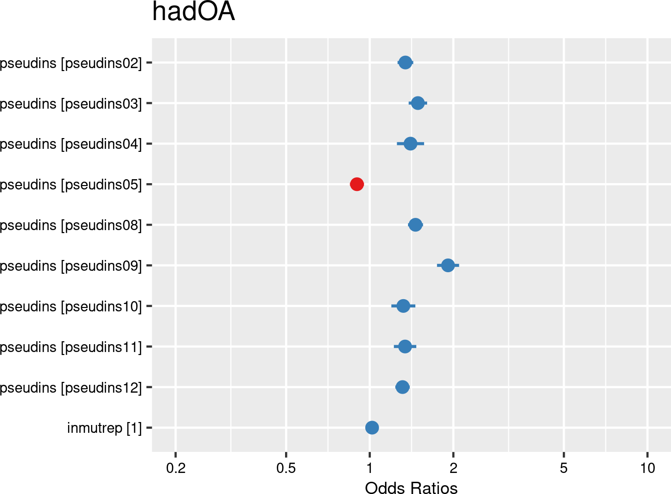

Insurer numbers (pseudonymised) were introduced as fixed effects, and companies and employees as random effects. The model is based on data of a sample of 50,000 workers. The model is adjusted for representativeness of the company (fixed effect inmutrep) regarding to sector, insurer and Flemish province.
According to Figure 3.157 (a) and Figure 3.157 (b), only insurers 2 and 9 show significantly lower odds ratios for having an OA refused by the insurer compared to the reference insurer (1). Other insurers do not show significant differences.
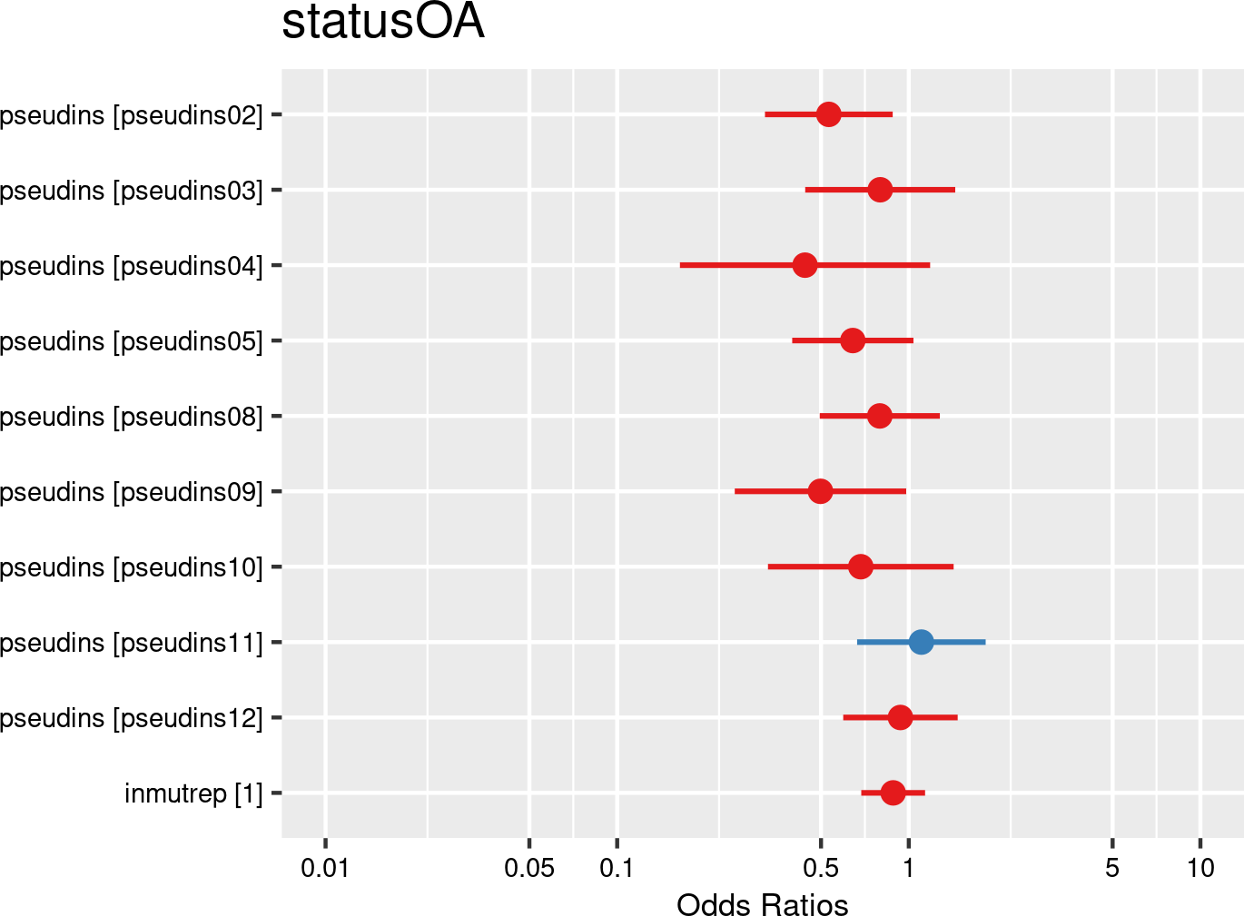

Insurer numbers (pseudonymised) were introduced as fixed effects, and companies and employees as random effects. The model is based on data of all employees. The model is adjusted for representativeness of the company (fixed effect inmutrep) regarding to sector, insurer and Flemish province.
According to Figure 3.158 (a) and Figure 3.158 (b), employees insured with insurers 2, 8, 10 and 11 have significantly higher odds of experiencing accepted commuting accidents compared to those insured with the reference insurer (1).
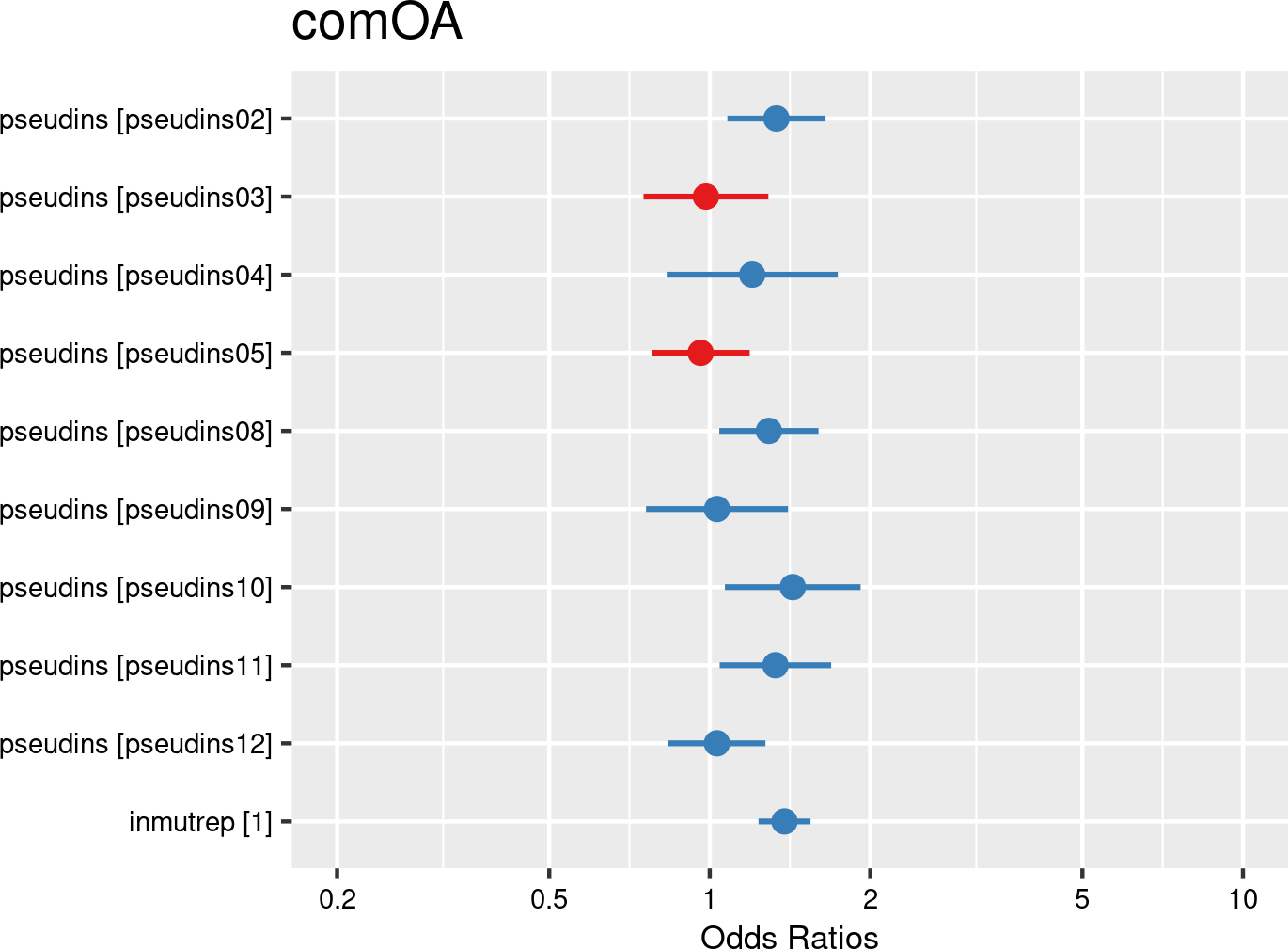

Insurer numbers (pseudonymised) were introduced as fixed effects, and companies and employees as random effects. The model is based on data of a sample of 50.000 workers. The model is adjusted for representativeness of the company (fixed effect inmutrep) regarding to sector, insurer and Flemish province.
Figure 3.159 (a) and Figure 3.159 (b) indicate that, for all insurers except insurer 5, the odds ratios for accepted workplace accidents are significantly higher compared to the reference insurer (1). Insurer 5 shows a notably lower odds ratio—approximately 10% less—while insurer 9 exhibits the highest odds ratio, at around 115% more. Given the substantial differences observed, further investigation is warranted (see Section 3.5) to assess whether these disparities persist when controlling for other variables.
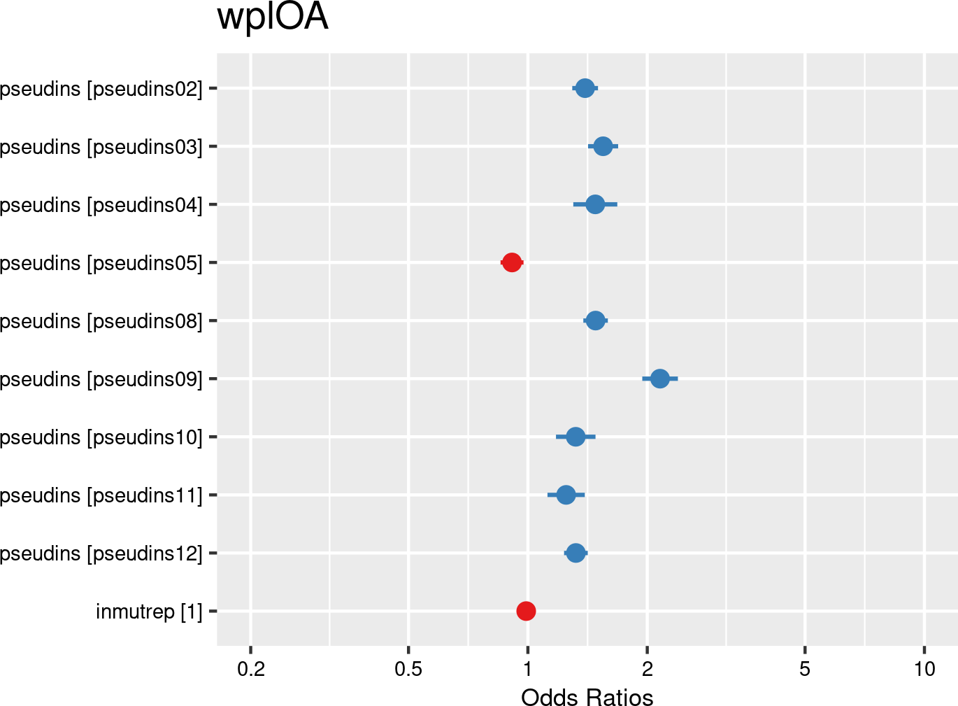

Insurer numbers (pseudonymised) were introduced as fixed effects, and companies and employees as random effects. The model is based on data of a sample of 50.000 workers. The model is adjusted for representativeness of the company (fixed effect inmutrep) regarding to sector, insurer and Flemish province.
Figure 3.160 (a) and Figure 3.160 (b) present a model estimating the frequency degree of OA at the company level, in contrast to earlier models that focused on individual employee accident probabilities. These figures show that all insurers -except insurer 5- have significantly higher frequency degree estimates compared to the reference insurer (1). Insurers 3 and 9 stand out with the highest frequency levels, while insurer 5 shows a notably lower result. Given the magnitude of these differences, further analysis is needed (see Section 3.5) to determine whether these patterns persist when controlling for other explanatory variables.
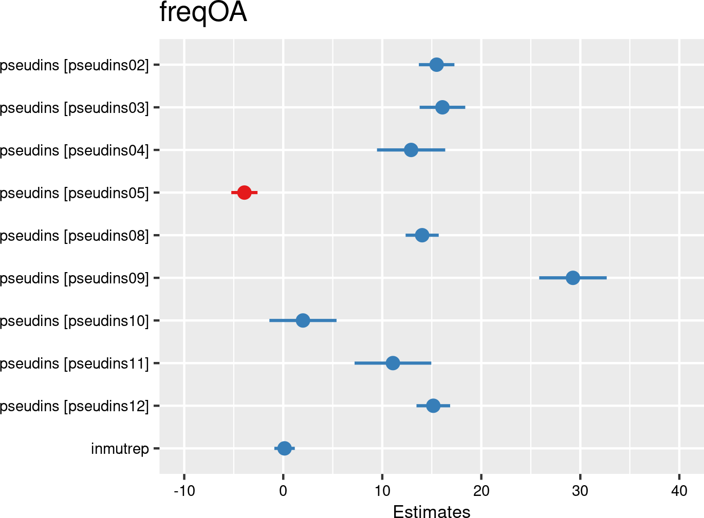

Insurer numbers (pseudonymised) proportions were introduced as fixed effects, and companies as random effects. The model is based on data of all mutual Liantis ESPP and PS customers. The model is adjusted for representativeness of the company (fixed effect inmutrep) regarding to sector, insurer and Flemish province.
Figure 3.161 (a) and Figure 3.161 (b) present a model estimating the chance for an accepted accident being serious (according to the definition of the Belgian law). These figures indicate that only insurers 10 and 11 show significantly lower odds ratios for having an accepted workplace OA classified as serious compared to the reference insurer (1). Other insurers do not show significant differences.
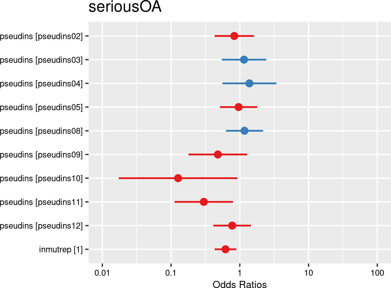

Insurer numbers (pseudonymised) were introduced as fixed effects, and companies and employees as random effects. The model is based on data of all mutual Liantis ESPP and PS customers. The model is adjusted for representativeness of the company (fixed effect inmutrep) regarding to sector, insurer and Flemish province.
Figure 3.162 (a) and Figure 3.162 (b) show that employees insured with insurers 2, 5 and 11 (and into a lesser extent 4 and 10) have significantly lower numbers of (FEDRIS validated) absence days associated with an accepted workplace OA compared to those insured with the reference insurer (1).
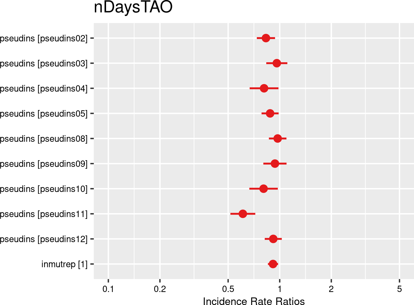

Insurer numbers (pseudonymised) were introduced as fixed effects, and companies and employees as random effects. The model is based on data of all mutual Liantis ESPP and PS customers. The model is adjusted for representativeness of the company (fixed effect inmutrep) regarding to sector, insurer and Flemish province.
Figure 3.163 (a) and Figure 3.163 (b) confirm that employees insured with insurers 2, 5 and 11 have significantly lower numbers of (Liantis PS calculated) absence days associated with an accepted workplace OA compared to those insured with the reference insurer (1).
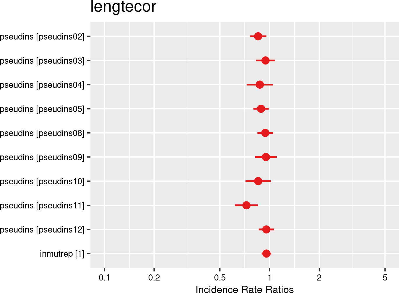

Insurer numbers (pseudonymised) were introduced as fixed effects, and companies and employees as random effects. The model is based on data of all mutual Liantis ESPP and PS customers. The model is adjusted for representativeness of the company (fixed effect inmutrep) regarding to sector, insurer and Flemish province.
Figure 3.164 (a) and Figure 3.164 (b) show that employees insured with insurer 2 have significantly lower direct wage costs associated with an accepted workplace OA compared to those insured with the reference insurer (1). In contrast, employees insured with insurer 9 exhibit significantly higher direct wage costs.
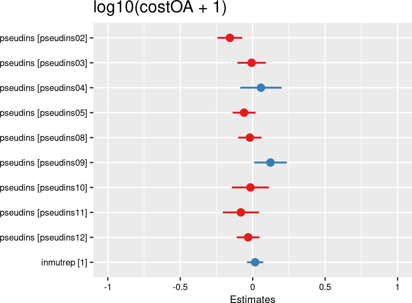

Insurer numbers (pseudonymised) were introduced as fixed effects, and companies and employees as random effects. The model is based on data of all mutual Liantis ESPP and PS customers. The model is adjusted for representativeness of the company (fixed effect inmutrep) regarding to sector, insurer and Flemish province.
The next 4 figures (Figure 3.165 (a) and Figure 3.165 (b), Figure 3.166 (a) and Figure 3.166 (b)) are displaying the results of models assessing the severity degree of a company in relation to its insurer. According to Figure 3.165 (a) and Figure 3.165 (b), insurers 2, 3, 8, 9 and 12 have significantly higher severity degree estimates compared to the reference insurer (1).
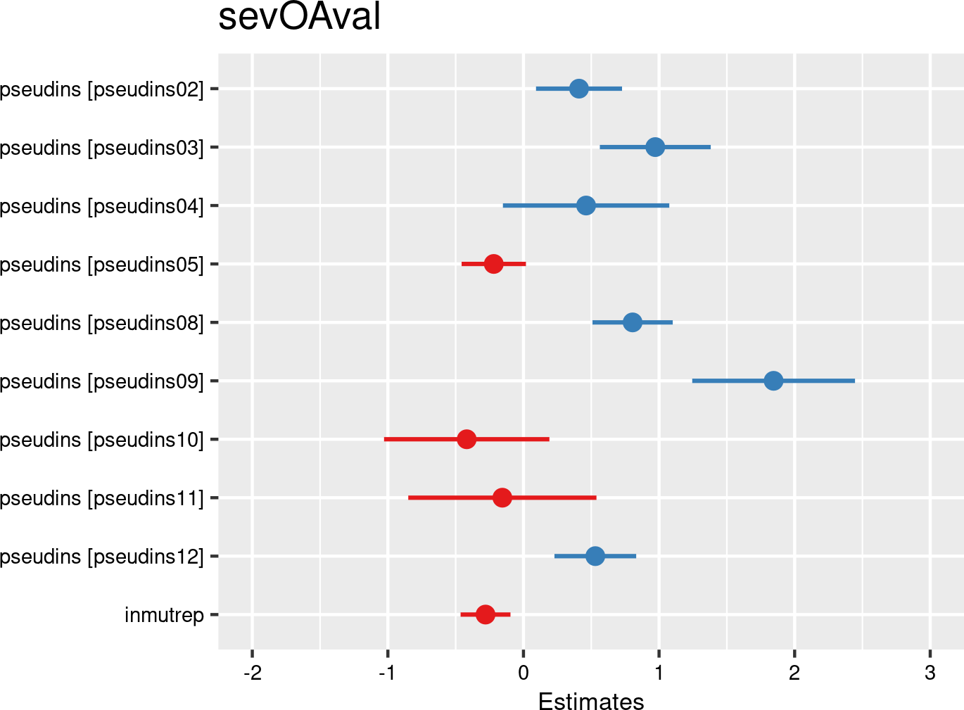

Insurer numbers (pseudonymised) proportions were introduced as fixed effects, and companies as random effects. The model is based on data of all mutual Liantis ESPP and PS customers. The model is adjusted for representativeness of the company (fixed effect inmutrep) regarding to sector, insurer and Flemish province.
Figure 3.166 (a) and Figure 3.166 (b) confirm the results of the previous model with validated days.
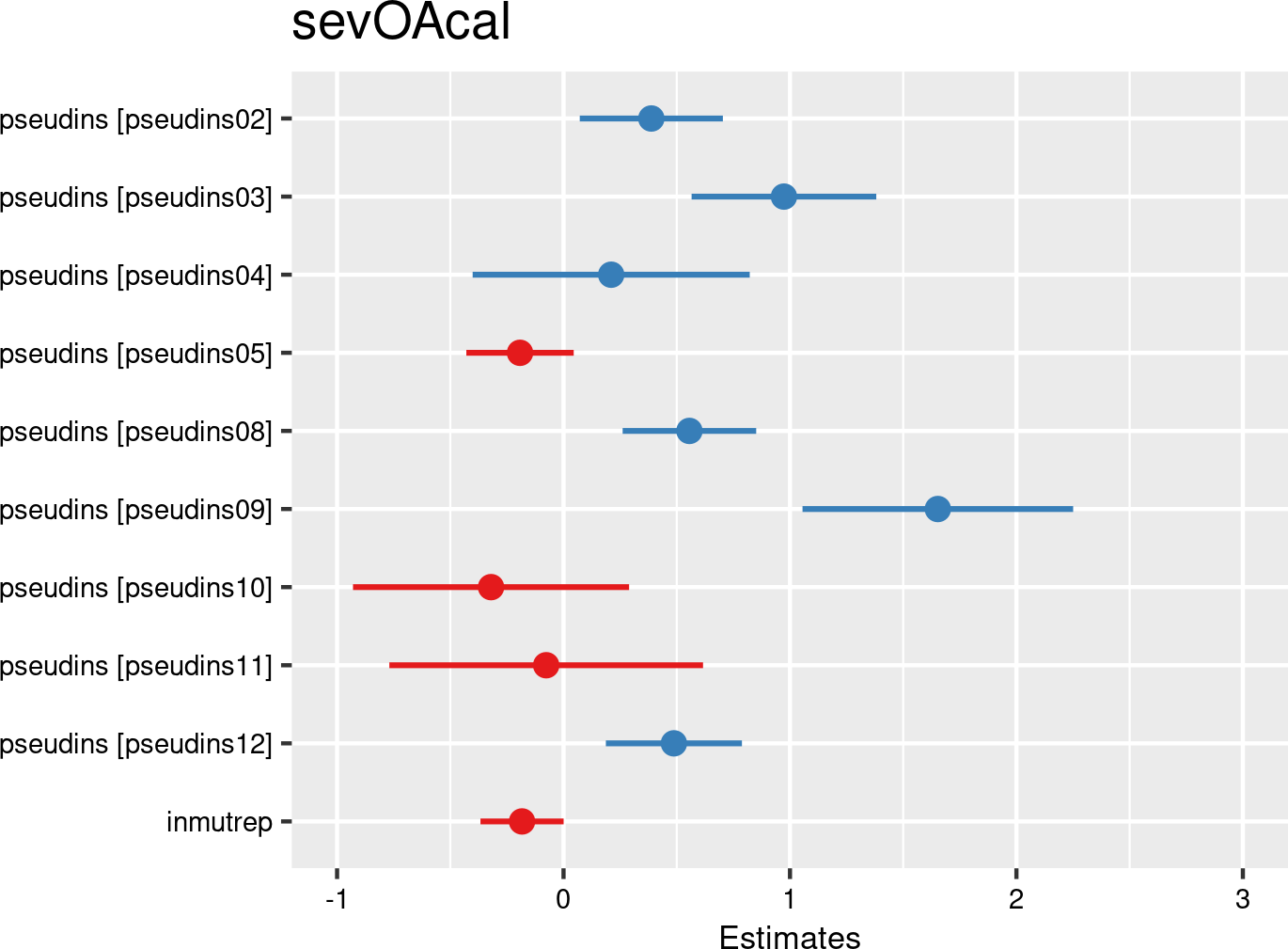

Insurer numbers (pseudonymised) proportions were introduced as fixed effects, and companies as random effects. The model is based on data of all mutual Liantis ESPP and PS customers. The model is adjusted for representativeness of the company (fixed effect inmutrep) regarding to sector, insurer and Flemish province.
3.4.3.6 Investments in prevention
Analysing the relationship between time invested in prevention and the occurrence of OA presents several methodological challenges, particularly when considering prevention time as a leading or predictive factor. To meaningfully assess this relationship, a sufficiently large and diverse dataset across multiple companies is required. This is especially important given that many organizations (fortunately) report zero occupational accidents, which limits the variability needed to detect patterns or vulnerabilities.
A preliminary aggregate-level analysis was performed using data exclusively from Liantis ESPP clients. This dataset comprises monthly records per company, including the number of employees, commuting and workplace OA notifications, and the total registered prevention time. Importantly, the recorded prevention time excludes any hours spent responding to OA after their occurrence. For further details on the time registration data, refer to Section 2.12.
Prior to aggregation, the dataset contains the total number of:
- employees (per company, per year, per month);
- commuting OA (per company, per year, per month);
- workplace OA (per company, per year, per month);
- hours invested by Liantis ESPP in preventive activities (per company, per year, per month).
By aggregating across all Liantis ESPP clients for each year and month, we construct a time series of 120 monthly totals for these four variables. To account for fluctuations in workforce size -whether due to internal changes within companies or shifts in the Liantis ESPP client portfolio- we normalize the three outcome variables (commuting OA, workplace OA, and time invested in prevention of OA) per 1,000 employees.
Figure 3.167 presents the three normalized time series: the number of commuting OA, the number of workplace OA, and the number of hours invested in prevention (excluding post-accident response time).
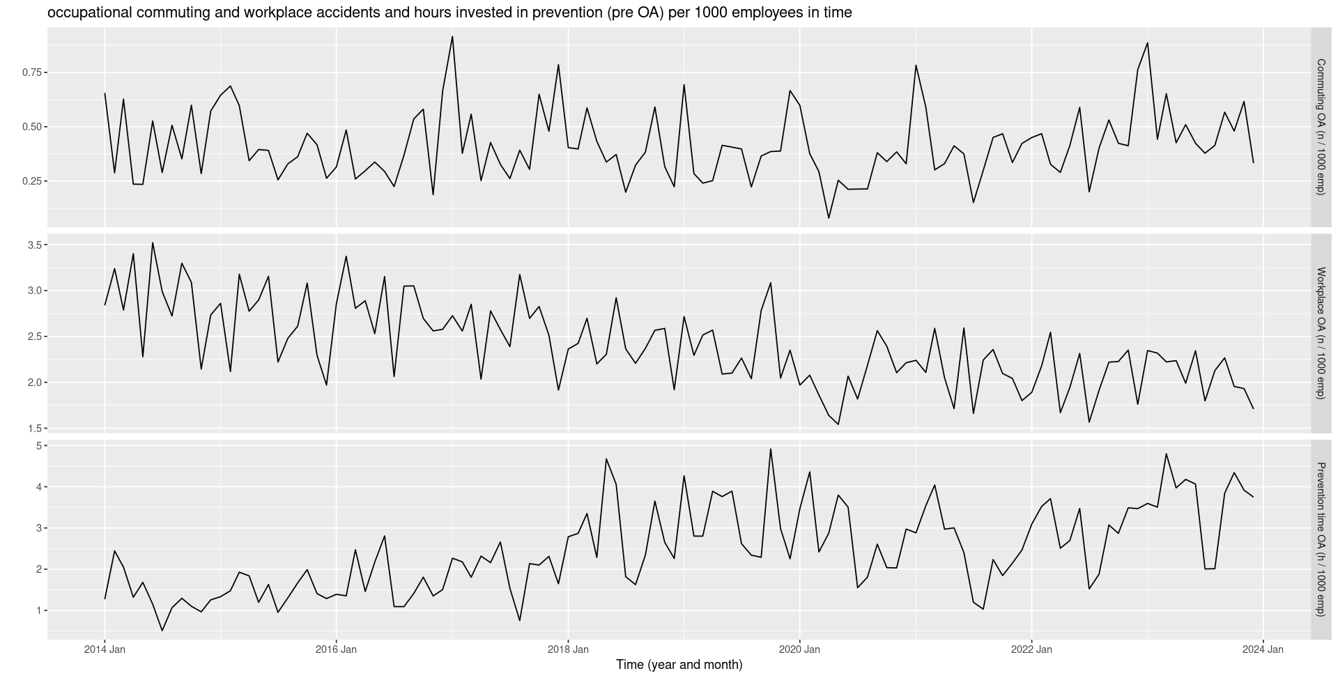
At first sight, a downward trend for workplace OA (middle panel) and an upward trend for time invested in prevention (lower panel) can be noticed, while the image for commuting OA seems less clear.
Due to the pronounced fluctuations and irregular patterns in the three timeseries, further interpretation can be challenging. To address this, a time series decomposition technique, Signal Extraction in Arima Time Series (SEATS) (Gómez & Maravall, 1997), is applied using the X_13ARIMA_SEATS function of the feasts package (O’Hara-Wild et al., 2024). The SEATS method separates the series into trend, seasonal, and irregular components, offering a clearer view of the underlying dynamics.
Results from the time series decomposition analyses using SEATS are presented in the upper parts of Figure 3.168, Figure 3.169, and Figure 3.170. The upper panel of each figure displays the same original time series as shown in Figure 3.167. The second panel shows the overall trend across the ten-year study.
- For commuting OA, a modest upward trend is observed starting from 2020 (see Figure 3.168 (a)).
- For workplace OA, a gradual and consistent downward trend is noticed over the ten-year period. The decline appears almost linear, suggesting a series of (long-term) improvements in workplace safety. These improvements may be attributed to enhanced preventive measures, better training, or changes in notification and reporting practices, being indicative of structural changes rather than short-term interventions (see Figure 3.169 (a)).
- For time invested in prevention of OA, the trend shows an increase from early 2014 to late 2019, followed by a decline until the end of 2021, and a renewed increase from late 2021 to the end of 2023. The impact of the Coronavirus Disease 2019 (COVID-19) pandemic, which is prominently visible in the raw data (upper panels comOA, wplOA, and prevOA of the three figures), only manifests as a prolonged two-year trend effect in the trend panel of Figure 3.170 (a)).
The lower parts of Figure 3.168, Figure 3.169, and Figure 3.170 display the seasonal components extracted by the SEATS method over the ten-year study period and correspond to the third panel of the upper part of each figure.
- For commuting OA, a pronounced seasonal effect is observed in January, with consistently elevated accident rates during this month (see Figure 3.168 (b)).
- For workplace OA, accident rates tend to peak in March, June, September, and October, while lower rates are typically seen in May, July, and December—possibly reflecting reduced activity during summer holidays or year-end periods. The seasonal pattern remains relatively stable across years, suggesting that certain months inherently carry higher risk, potentially due to weather conditions, workload fluctuations, or staffing dynamics (see Figure 3.169 (b)).
- For time invested in prevention of OA, seasonal peaks are consistently observed in the first quarter of each year, followed by a dip around mid-year (see Figure 3.170 (b)). This pattern may reflect organizational planning cycles, with increased allocation of resources to prevention activities early in the year—possibly linked to budget planning or strategic initiatives—and a quieter period during July and August.
The irregular component (fourth and lowest panel of the upper part of Figure 3.168, Figure 3.169, and Figure 3.170) captures short-term fluctuations that cannot be explained by trend or seasonality. These may be due to isolated incidents or anomalies, large and sudden changes in reporting or data collection, external shocks like policy changes or pandemics,…
Investments in prevention increase, workplace occupational accidents numbers decrease
Time series decomposition using SEATS reveals distinct seasonal peaks in both commuting and workplace occupational accidents, suggesting potential for targeted interventions during high-risk months. The analysis confirms that the observed patterns are not purely random. Notably, a slight upward trend in commuting occupational accidents emerges from mid-2020 onward. In contrast, workplace OA show a clear and encouraging downward trend, which appears to coincide with a collective increase in preventive investments across the Liantis ESPP client portfolio. This raises the question whether continued investment in prevention could sustain or further reinforce both trajectories.
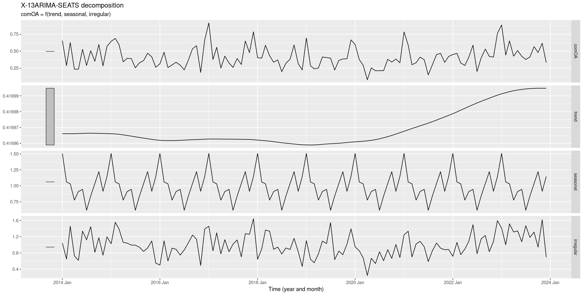
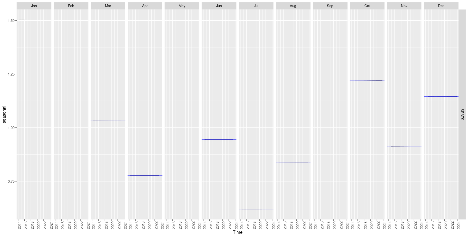
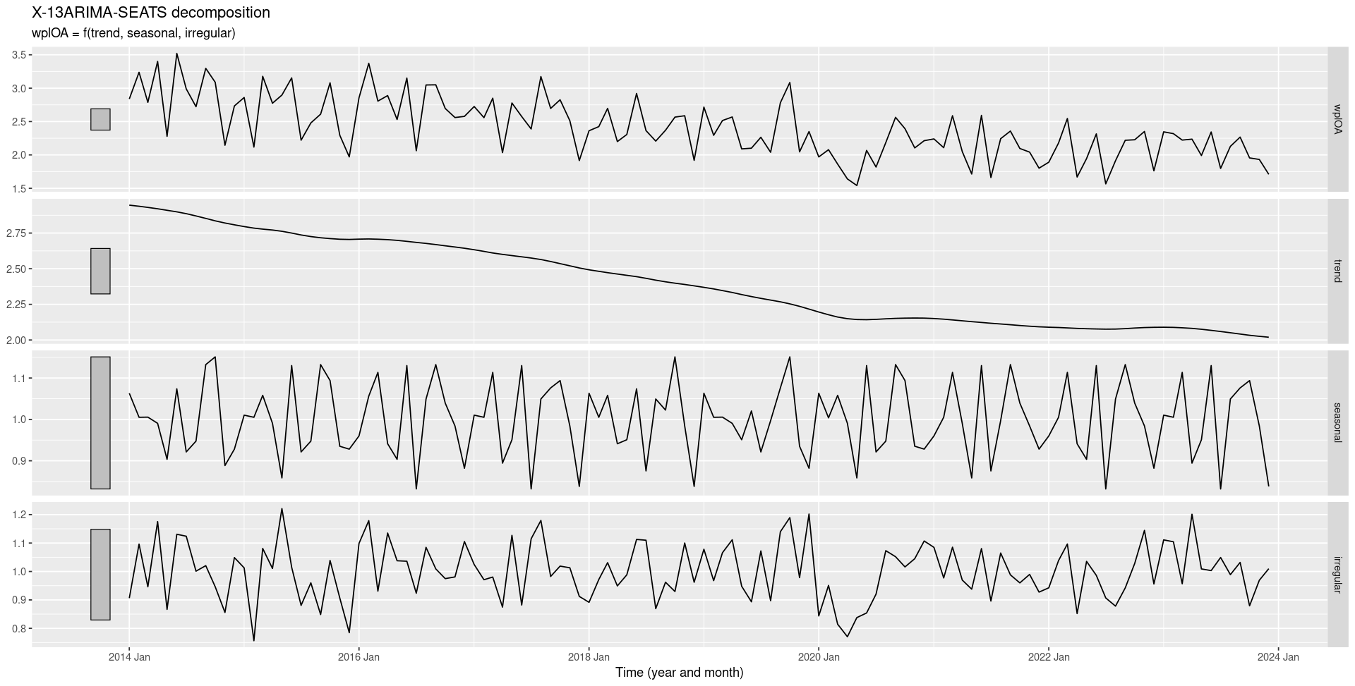
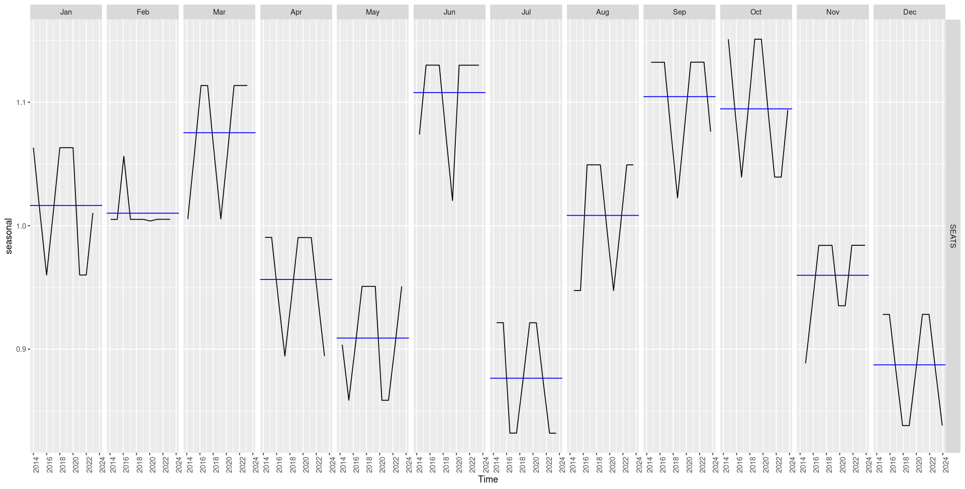
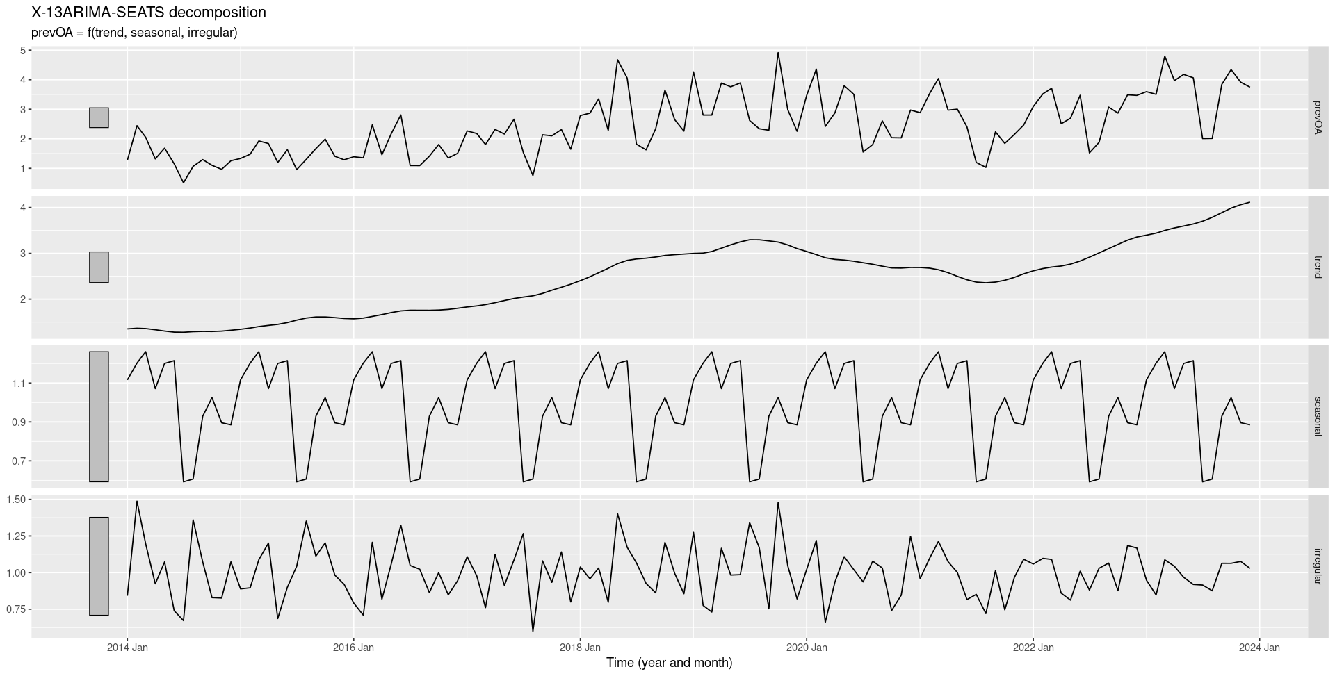

Although it is impossible to establish any causal relationships from the raw and decomposed time series, the normalised increased time invested in prevention coincides with lower normalised numbers of workplace OA (but not with lower numbers of commuting OA).
Due to the limited number of observations (120 months with aggregated data available in the dataset), it is not possible to conduct a robust statistical analysis.
A scatterplot of the 120 data points (see Figure 3.171) however confirms (in blue) the negative relation between investment in prevention and workplace OA observed in time series trends: a higher amount of time invested in prevention OA is related to a lower number of workplace OA, but not to a lower number of commuting OA (in red). While these observations are based on a simplified analysis, they offer an indication that prevention investments might have a positive impact on workplace OA occurrence.
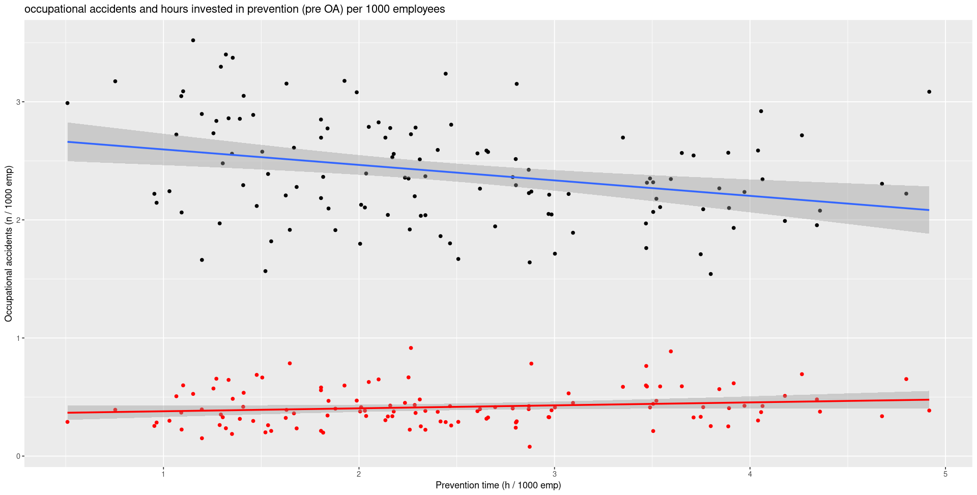
Again, it is important to emphasize that this analysis does not allow for causal inference. We cannot conclude, based on this data alone, that companies investing more time in prevention necessarily experience fewer workplace OA. The observed patterns warrant further investigation using more advanced statistical techniques.
Prevention investments might have a positive impact on workplace OA occurrence
While our initial findings suggest a potential link between time invested in prevention and worplace occupational accident notification rates, the limitations of the dataset and the aggregate nature of the analysis mean that no definitive conclusions can be drawn at this stage. Future research should aim to explore this relationship in greater depth, using robust modelling approaches and more detailed and high quality datasets.
3.4.4 Sectoral differences
3.4.4.1 Section NACE-BEL 2008
3.4.4.1.1 Descriptives
Both NSSO and FEDRIS provide statistics on the sector of the employee (NSSO section level, 1 digit and FEDRIS division level, 2 digits). From Liantis PS data it is also possible to derive the section of the employer through the subclass level (5 digits) of an employer. The notification in many cases also contains the subclass level of the employer (5 digits). Since this information is also present in the notification information passed through to Liantis, the fit between the derived section of the employer of an employee experiencing an OA can be compared with the corresponding section derived from the original notification of the accident.
From Figure 3.172 we learn that the sections derived from Liantis PS data and FEDRIS data are highly comparable when both are available. The correlation between the two datasets is 98%. This suggests that the sections derived from Liantis PS data align well with those in FEDRIS data, making them suitable for further analysis.
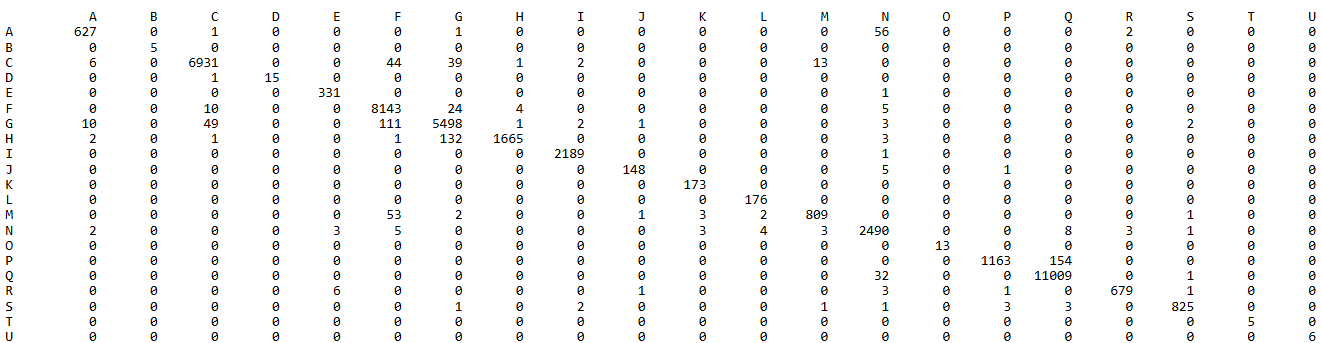
all accepted occupational accidents
| nace | rszall | rszpriv | liaall | fedrisall | totalnot | totalnotmut | totalnotrepmutflan |
|---|---|---|---|---|---|---|---|
| A | 953206 | 953206 | 238640 | 1720 | 1190 | 774 | 234 |
| B | 96322 | 96322 | 486 | 330 | 405 | 51 | NA |
| C | 18938833 | 18938253 | 1859279 | 84924 | 43836 | 9377 | 4001 |
| D | 742516 | 699656 | 5600 | 1251 | 158 | 14 | NA |
| E | 1094598 | 853266 | 56820 | 4887 | 3254 | 565 | NA |
| F | 8197964 | 8197964 | 1754346 | 27208 | 28060 | 12006 | 2747 |
| G | 19742342 | 19742342 | 2965033 | 57134 | 17293 | 7518 | 2082 |
| H | 9119531 | 7503286 | 545779 | 36513 | 11277 | 3121 | 1258 |
| I | 4471088 | 4470459 | 2537607 | 10891 | 4208 | 2875 | 498 |
| J | 4317974 | 4121508 | 211759 | 7154 | 710 | 235 | 91 |
| K | 4825380 | 4823556 | 246944 | 9494 | 1580 | 217 | 60 |
| L | 847838 | 841704 | 169100 | 1499 | 470 | 210 | 57 |
| M | 6851246 | 6780059 | 782264 | 13135 | 2273 | 975 | 301 |
| N | 15699074 | 15560973 | 924668 | 63615 | 8486 | 3617 | 1155 |
| O | 15493922 | 7320334 | 9007 | 3057 | 9878 | 15 | NA |
| P | 15957634 | 6642834 | 701217 | 6421 | 2819 | 1677 | 908 |
| Q | 21268309 | 20726706 | 2621790 | 73128 | 52179 | 14876 | 11719 |
| R | 1460856 | 1439992 | 248602 | 4731 | 2670 | 1272 | 354 |
| S | 2815390 | 2813402 | 631306 | 5988 | 2527 | 1266 | 327 |
| T | 147863 | 147863 | 11613 | 58 | 18 | 9 | NA |
| U | 126256 | 126256 | 12224 | 221 | 7 | 7 | NA |
| NA | NA | NA | 1521782 | 439697 | 1921 | 558 | 238 |
| nace | percrszall | percrszpriv | percliaall | percfedrisall | perctotalnot | perctotalnotmut | perctotalnotrepmutflan |
|---|---|---|---|---|---|---|---|
| A | 0.6 | 0.7 | 1.4 | 0.4 | 0.6 | 1.3 | 0.9 |
| B | 0.1 | 0.1 | 0.0 | 0.1 | 0.2 | 0.1 | NA |
| C | 12.4 | 14.3 | 11.2 | 20.5 | 22.7 | 15.5 | 15.5 |
| D | 0.5 | 0.5 | 0.0 | 0.3 | 0.1 | 0.0 | NA |
| E | 0.7 | 0.6 | 0.3 | 1.2 | 1.7 | 0.9 | NA |
| F | 5.4 | 6.2 | 10.6 | 6.6 | 14.5 | 19.8 | 10.7 |
| G | 12.9 | 14.9 | 17.9 | 13.8 | 8.9 | 12.4 | 8.1 |
| H | 6.0 | 5.7 | 3.3 | 8.8 | 5.8 | 5.1 | 4.9 |
| I | 2.9 | 3.4 | 15.3 | 2.6 | 2.2 | 4.7 | 1.9 |
| J | 2.8 | 3.1 | 1.3 | 1.7 | 0.4 | 0.4 | 0.4 |
| K | 3.2 | 3.6 | 1.5 | 2.3 | 0.8 | 0.4 | 0.2 |
| L | 0.6 | 0.6 | 1.0 | 0.4 | 0.2 | 0.3 | 0.2 |
| M | 4.5 | 5.1 | 4.7 | 3.2 | 1.2 | 1.6 | 1.2 |
| N | 10.2 | 11.7 | 5.6 | 15.4 | 4.4 | 6.0 | 4.5 |
| O | 10.1 | 5.5 | 0.1 | 0.7 | 5.1 | 0.0 | NA |
| P | 10.4 | 5.0 | 4.2 | 1.6 | 1.5 | 2.8 | 3.5 |
| Q | 13.9 | 15.6 | 15.9 | 17.7 | 27.0 | 24.5 | 45.4 |
| R | 1.0 | 1.1 | 1.5 | 1.1 | 1.4 | 2.1 | 1.4 |
| S | 1.8 | 2.1 | 3.8 | 1.4 | 1.3 | 2.1 | 1.3 |
| T | 0.1 | 0.1 | 0.1 | 0.0 | 0.0 | 0.0 | NA |
| U | 0.1 | 0.1 | 0.1 | 0.1 | 0.0 | 0.0 | NA |
| NA | NA | NA | NA | NA | NA | NA | NA |
commuting accepted occupational accidents
| nace | rszall | rszpriv | liaall | fedrisall | totalnot | totalnotmut | totalnotrepmutflan |
|---|---|---|---|---|---|---|---|
| A | 953206 | 953206 | 238640 | 677 | 80 | 54 | 19 |
| B | 96322 | 96322 | 486 | 102 | 21 | NA | NA |
| C | 18938833 | 18938253 | 1859279 | 31170 | 4588 | 940 | 402 |
| D | 742516 | 699656 | 5600 | 1007 | 84 | 1 | NA |
| E | 1094598 | 853266 | 56820 | 1041 | 268 | 33 | NA |
| F | 8197964 | 8197964 | 1754346 | 8040 | 1532 | 591 | 152 |
| G | 19742342 | 19742342 | 2965033 | 28330 | 2395 | 1187 | 391 |
| H | 9119531 | 7503286 | 545779 | 12996 | 1062 | 150 | 61 |
| I | 4471088 | 4470459 | 2537607 | 5888 | 658 | 467 | 68 |
| J | 4317974 | 4121508 | 211759 | 5703 | 320 | 113 | 50 |
| K | 4825380 | 4823556 | 246944 | 8897 | 904 | 105 | 23 |
| L | 847838 | 841704 | 169100 | 1030 | 99 | 41 | 18 |
| M | 6851246 | 6780059 | 782264 | 10219 | 720 | 341 | 110 |
| N | 15699074 | 15560973 | 924668 | 42351 | 1660 | 717 | 311 |
| O | 15493922 | 7320334 | 9007 | 2586 | 2007 | 3 | NA |
| P | 15957634 | 6642834 | 701217 | 4294 | 567 | 367 | 182 |
| Q | 21268309 | 20726706 | 2621790 | 52663 | 10130 | 2922 | 2152 |
| R | 1460856 | 1439992 | 248602 | 2045 | 206 | 97 | 24 |
| S | 2815390 | 2813402 | 631306 | 4706 | 757 | 393 | 112 |
| T | 147863 | 147863 | 11613 | 36 | 1 | 1 | NA |
| U | 126256 | 126256 | 12224 | 138 | 4 | 4 | NA |
| NA | NA | NA | 1521782 | 228699 | 324 | 72 | 37 |
| nace | percrszall | percrszpriv | percliaall | percfedrisall | perctotalnot | perctotalnotmut | perctotalnotrepmutflan |
|---|---|---|---|---|---|---|---|
| A | 0.6 | 0.7 | 1.4 | 0.3 | 0.3 | 0.6 | 0.5 |
| B | 0.1 | 0.1 | 0.0 | 0.0 | 0.1 | NA | NA |
| C | 12.4 | 14.3 | 11.2 | 13.9 | 16.3 | 11.0 | 9.9 |
| D | 0.5 | 0.5 | 0.0 | 0.4 | 0.3 | 0.0 | NA |
| E | 0.7 | 0.6 | 0.3 | 0.5 | 1.0 | 0.4 | NA |
| F | 5.4 | 6.2 | 10.6 | 3.6 | 5.5 | 6.9 | 3.7 |
| G | 12.9 | 14.9 | 17.9 | 12.7 | 8.5 | 13.9 | 9.6 |
| H | 6.0 | 5.7 | 3.3 | 5.8 | 3.8 | 1.8 | 1.5 |
| I | 2.9 | 3.4 | 15.3 | 2.6 | 2.3 | 5.5 | 1.7 |
| J | 2.8 | 3.1 | 1.3 | 2.5 | 1.1 | 1.3 | 1.2 |
| K | 3.2 | 3.6 | 1.5 | 4.0 | 3.2 | 1.2 | 0.6 |
| L | 0.6 | 0.6 | 1.0 | 0.5 | 0.4 | 0.5 | 0.4 |
| M | 4.5 | 5.1 | 4.7 | 4.6 | 2.6 | 4.0 | 2.7 |
| N | 10.2 | 11.7 | 5.6 | 18.9 | 5.9 | 8.4 | 7.6 |
| O | 10.1 | 5.5 | 0.1 | 1.2 | 7.2 | 0.0 | NA |
| P | 10.4 | 5.0 | 4.2 | 1.9 | 2.0 | 4.3 | 4.5 |
| Q | 13.9 | 15.6 | 15.9 | 23.5 | 36.1 | 34.3 | 52.8 |
| R | 1.0 | 1.1 | 1.5 | 0.9 | 0.7 | 1.1 | 0.6 |
| S | 1.8 | 2.1 | 3.8 | 2.1 | 2.7 | 4.6 | 2.7 |
| T | 0.1 | 0.1 | 0.1 | 0.0 | 0.0 | 0.0 | NA |
| U | 0.1 | 0.1 | 0.1 | 0.1 | 0.0 | 0.0 | NA |
| NA | NA | NA | NA | NA | NA | NA | NA |
workplace accepted occupational accidents
| nace | rszall | rszpriv | liaall | fedrisall | totalnot | totalnotmut | totalnotrepmutflan |
|---|---|---|---|---|---|---|---|
| A | 953206 | 953206 | 238640 | 1043 | 1110 | 720 | 215 |
| B | 96322 | 96322 | 486 | 228 | 384 | 51 | NA |
| C | 18938833 | 18938253 | 1859279 | 53754 | 39248 | 8437 | 3599 |
| D | 742516 | 699656 | 5600 | 244 | 74 | 13 | NA |
| E | 1094598 | 853266 | 56820 | 3846 | 2986 | 532 | NA |
| F | 8197964 | 8197964 | 1754346 | 19168 | 26528 | 11415 | 2595 |
| G | 19742342 | 19742342 | 2965033 | 28804 | 14898 | 6331 | 1691 |
| H | 9119531 | 7503286 | 545779 | 23517 | 10215 | 2971 | 1197 |
| I | 4471088 | 4470459 | 2537607 | 5003 | 3550 | 2408 | 430 |
| J | 4317974 | 4121508 | 211759 | 1451 | 390 | 122 | 41 |
| K | 4825380 | 4823556 | 246944 | 597 | 676 | 112 | 37 |
| L | 847838 | 841704 | 169100 | 469 | 371 | 169 | 39 |
| M | 6851246 | 6780059 | 782264 | 2916 | 1553 | 634 | 191 |
| N | 15699074 | 15560973 | 924668 | 21264 | 6826 | 2900 | 844 |
| O | 15493922 | 7320334 | 9007 | 471 | 7871 | 12 | NA |
| P | 15957634 | 6642834 | 701217 | 2127 | 2252 | 1310 | 726 |
| Q | 21268309 | 20726706 | 2621790 | 20465 | 42049 | 11954 | 9567 |
| R | 1460856 | 1439992 | 248602 | 2686 | 2464 | 1175 | 330 |
| S | 2815390 | 2813402 | 631306 | 1282 | 1770 | 873 | 215 |
| T | 147863 | 147863 | 11613 | 22 | 17 | 8 | NA |
| U | 126256 | 126256 | 12224 | 83 | 3 | 3 | NA |
| NA | NA | NA | 1521782 | 210998 | 1597 | 486 | 201 |
| nace | percrszall | percrszpriv | percliaall | percfedrisall | perctotalnot | perctotalnotmut | perctotalnotrepmutflan |
|---|---|---|---|---|---|---|---|
| A | 0.6 | 0.7 | 1.4 | 0.6 | 0.7 | 1.4 | 1.0 |
| B | 0.1 | 0.1 | 0.0 | 0.1 | 0.2 | 0.1 | NA |
| C | 12.4 | 14.3 | 11.2 | 28.4 | 23.8 | 16.2 | 16.6 |
| D | 0.5 | 0.5 | 0.0 | 0.1 | 0.0 | 0.0 | NA |
| E | 0.7 | 0.6 | 0.3 | 2.0 | 1.8 | 1.0 | NA |
| F | 5.4 | 6.2 | 10.6 | 10.1 | 16.1 | 21.9 | 11.9 |
| G | 12.9 | 14.9 | 17.9 | 15.2 | 9.0 | 12.1 | 7.8 |
| H | 6.0 | 5.7 | 3.3 | 12.4 | 6.2 | 5.7 | 5.5 |
| I | 2.9 | 3.4 | 15.3 | 2.6 | 2.1 | 4.6 | 2.0 |
| J | 2.8 | 3.1 | 1.3 | 0.8 | 0.2 | 0.2 | 0.2 |
| K | 3.2 | 3.6 | 1.5 | 0.3 | 0.4 | 0.2 | 0.2 |
| L | 0.6 | 0.6 | 1.0 | 0.2 | 0.2 | 0.3 | 0.2 |
| M | 4.5 | 5.1 | 4.7 | 1.5 | 0.9 | 1.2 | 0.9 |
| N | 10.2 | 11.7 | 5.6 | 11.2 | 4.1 | 5.6 | 3.9 |
| O | 10.1 | 5.5 | 0.1 | 0.2 | 4.8 | 0.0 | NA |
| P | 10.4 | 5.0 | 4.2 | 1.1 | 1.4 | 2.5 | 3.3 |
| Q | 13.9 | 15.6 | 15.9 | 10.8 | 25.4 | 22.9 | 44.1 |
| R | 1.0 | 1.1 | 1.5 | 1.4 | 1.5 | 2.3 | 1.5 |
| S | 1.8 | 2.1 | 3.8 | 0.7 | 1.1 | 1.7 | 1.0 |
| T | 0.1 | 0.1 | 0.1 | 0.0 | 0.0 | 0.0 | NA |
| U | 0.1 | 0.1 | 0.1 | 0.0 | 0.0 | 0.0 | NA |
| NA | NA | NA | NA | NA | NA | NA | NA |
3.4.4.1.2 Models
The following Table 3.115 table summarizes the results of the models assessing the relationship between NACE-BEL 2008 categories and the several outcomes related to OAs. Below the table, details are provided about the data used for the analyses. The results of the nine models are then presented both graphically and in a table.
| catnace | chance to notify | chance on refusal | chance commuting | chance workplace | freq degree | chance serious | nDays TAO V/C | cost | sev degree V/C |
|---|---|---|---|---|---|---|---|---|---|
| A | REF | REF | REF | REF | ns | REF | REF | REF | REF |
| C | ns | ns | ns | ns | > | ns | ns | > | </< |
| F | > | ns | ns | > | > | ns | ns | > | >/ns |
| G | < | ns | ns | < | < | ns | ns | ns | </< |
| H | ns | ns | ns | ns | ns | ns | >/ns | > | ns |
| I | < | ns | ns | < | < | ns | </< | < | </< |
| J | < | ns | ns | < | < | ns | </ns | < | </< |
| K | < | ns | ns | < | < | ns | ns | < | </< |
| L | < | ns | ns | < | < | ns | </ns | ns | </< |
| M | < | ns | ns | < | < | ns | </< | < | </< |
| N | ns | ns | > | ns | ns | ns | ns/< | > | ns |
| P | < | ns | ns | < | < | ns | </< | < | </< |
| Q | < | ns | > | < | < | < | </< | < | </< |
| R | < | ns | ns | < | < | ns | ns | < | </< |
| S | < | ns | ns | < | < | ns | </ns | < | </< |
| occur | accept | occur | occur | occur | severe | severe | severe | severe | |
| empl | empl | empl | empl | comp | empl | empl | empl | comp | |
| c/w all | c/w ref | c acc | w acc | w acc | w acc | w acc | w acc | w acc |
- occur: data include all workers, chance for occurrence is calculated for the outcome
- accept: data include only workers with a notification of OA
- severe: data include only workers with an accepted OA
- c/w all: commuting and workplace accidents, including refused and accidents without decisions
- c/w ref: accepted or refused commuting and workplace accidents
- c acc: accepted commuting accidents
- w acc: accepted workplace accidents
- empl: the outcome is situated at the individual level
- comp: the outcome is situated at the company level
- nDaysTAO: number of days absenteeism related to the OA
- V/C: Validated number of days (available from FEDRIS) / Calculated number of days (based on the Liantis PS data)
Section NACE-BEL 2008 and occupational accidents
- Compared to reference sector A (Agriculture, forestry and fishing)
- Likelihoods to notify seem to be higher in sector F (Construction) and equal or lower in almost all other sectors
- Likelihoods for refusal do not seem to differ significantly between sectors
- Likelihoods for experiencing commuting accidents appear to be higher in sectors N (Administrative and support service activities) and Q (Human health and social work activities)
- Likelihoods for experiencing workplace accidents appear to be higher in sector F (Construction) and lower in almost all other sectors
- Frequency degrees at company level appear to be higher in sectors C (Manufacturing) and F (Construction)
- Likelihoods for serious accidents only seems to be lower in sector Q (Human health and social work activities)
- Number of absence days associated with an accepted workplace accident seem to be lower in M (Professional, scientific and technical activities) and higher in H (Transportation and storage)
- Costs appear to be higher in sectors C (Manufacturing), F (Construction) and H (Transportation and storage) and lower in almost all other sectors
- Severity degrees at company level appear to be higher in sectors F (Construction) and lower in almost all other sectors
- influence of sector as determinant needs to be further assessed in the multivariable analysis (see Section 3.5) to clarify whether the observed differences persist when adjusting for other variables
From Figure 3.173 (a) and Figure 3.173 (b) we learn that, compared to the reference sector A (Agriculture, forestry and fishing), sector F (Construction) shows significantly higher odds ratios for notifying an OA, while most other sectors exhibit significantly lower odds ratios.
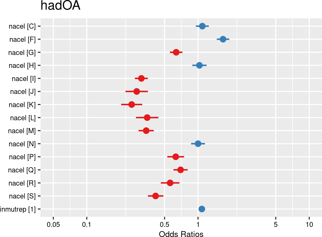

NACE-BEL 2008 Level 1 categories were introduced as fixed effects, and companies and employees as random effects. The model is based on data of a sample of 50,000 workers. The model is adjusted for representativeness of the company (fixed effect inmutrep) regarding to sector, size and Flemish province.
According to Figure 3.174 (a) and Figure 3.174 (b), the sector of a company is not significantly associated with the odds of having a reported OA refused by the insurer.
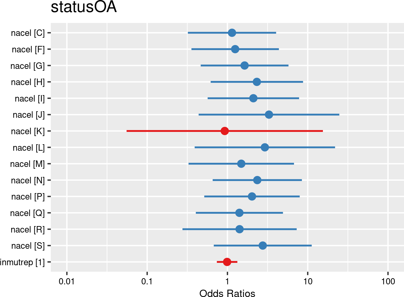

NACE-BEL 2008 Level 1 categories were introduced as fixed effects, and companies and employees as random effects. The model is based on data of all employees. The model is adjusted for representativeness of the company (fixed effect inmutrep) regarding to sector, size and Flemish province.
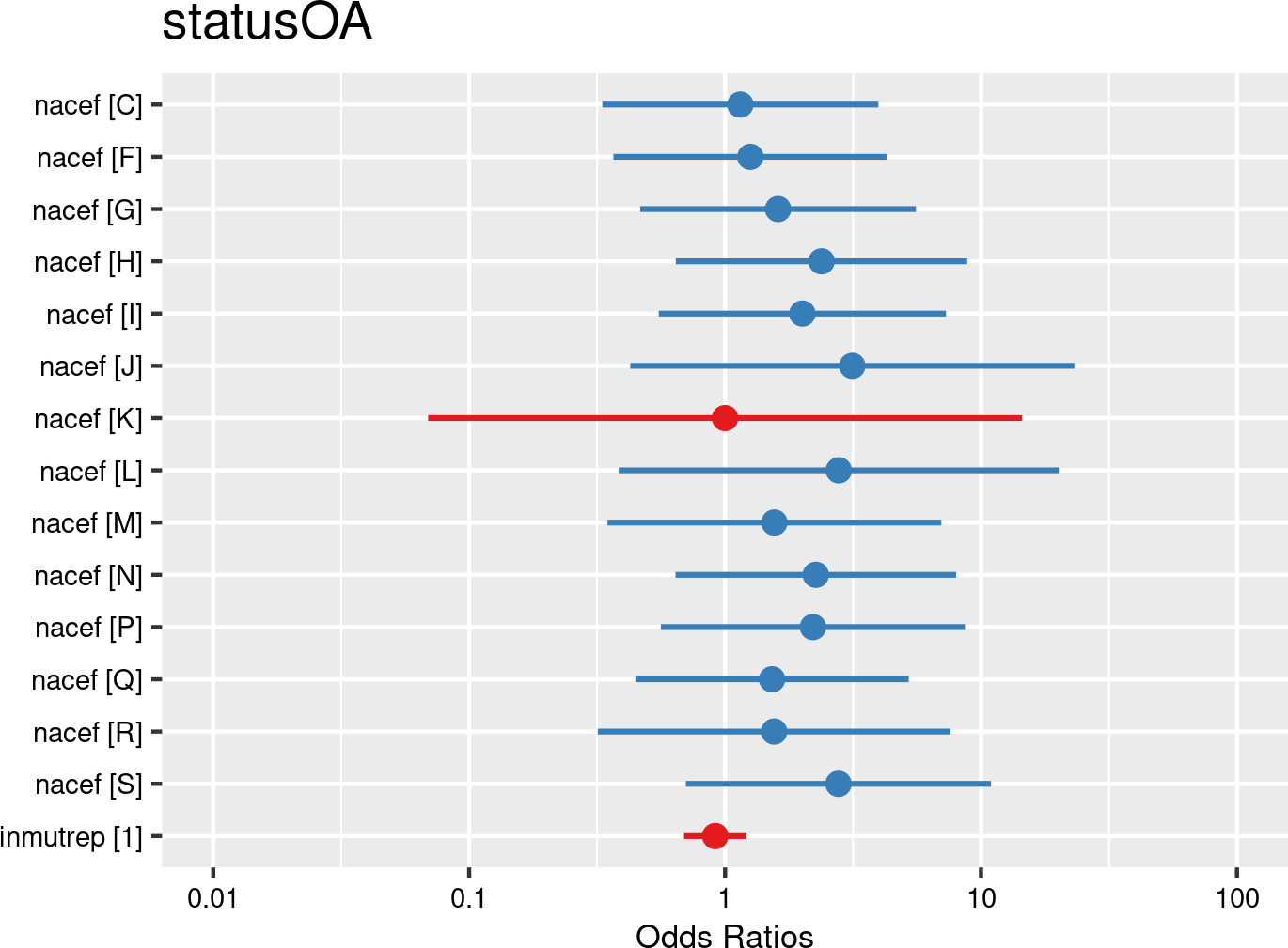

NACE-BEL 2008 Level 1 categories were introduced as fixed effects, and companies and employees as random effects. The model is based on data of all employees. The model is adjusted for representativeness of the company (fixed effect inmutrep) regarding to sector, size and Flemish province.
Linear mixed-effects model 1.1 assessing the impact of NACE-BEL 2008 Level 1 categories on the probability of a reported OA being refused by the insurer
According to Figure 3.175 (a) and Figure 3.175 (b), the likelihoods for experiencing commuting accidents appear to be higher in sectors N (Administrative and support service activities) and Q (Human health and social work activities) compared to the reference sector A (Agriculture, forestry and fishing).
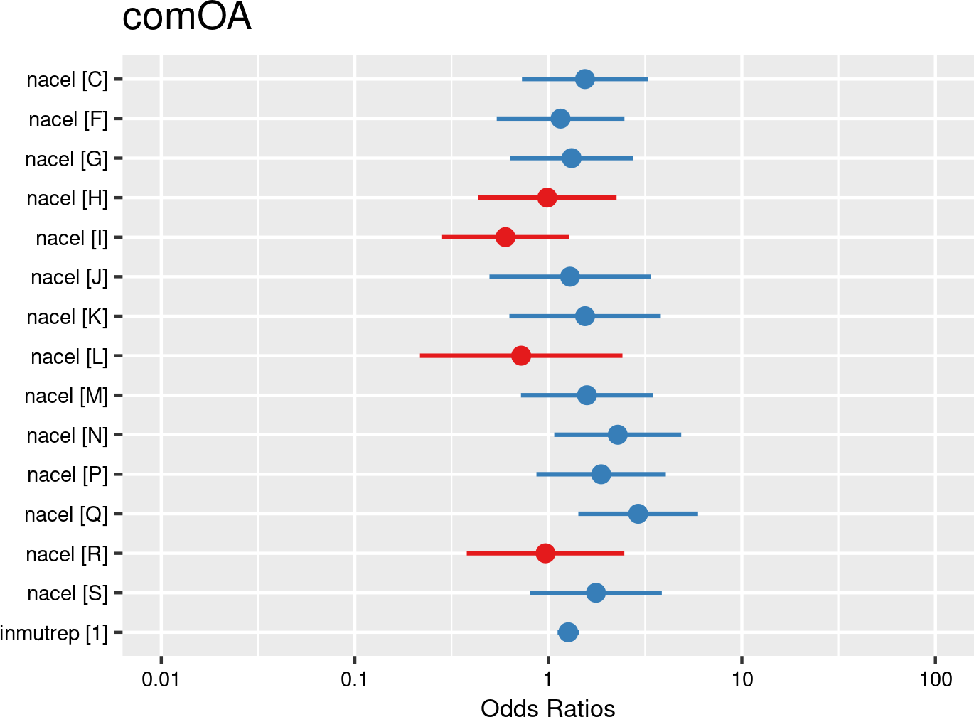

NACE-BEL 2008 Level 1 categories were introduced as fixed effects, and companies and employees as random effects. The model is based on data of a sample of 50.000 workers. The model is adjusted for representativeness of the company (fixed effect inmutrep) regarding to sector, size and Flemish province.
Figure 3.176 (a) and Figure 3.176 (b) show that, compared to the reference sector A (Agriculture, forestry and fishing), sector F (Construction) exhibits significantly higher odds ratios for accepted workplace accidents, while most other sectors display significantly lower odds ratios.
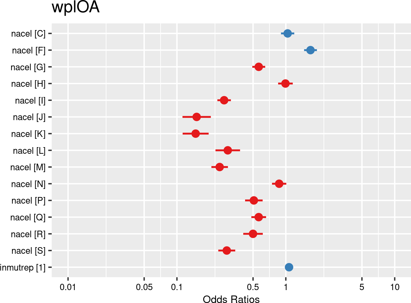

NACE-BEL 2008 Level 1 categories were introduced as fixed effects, and companies and employees as random effects. The model is based on data of a sample of 50.000 workers. The model is adjusted for representativeness of the company (fixed effect inmutrep) regarding to sector, size and Flemish province.
Figure 3.177 (a) and Figure 3.177 (b) present a model estimating the frequency degree of OA at the company level. These figures indicate that sectors C (Manufacturing) and F (Construction) have significantly higher frequency degree estimates compared to the reference sector A (Agriculture, forestry and fishing).
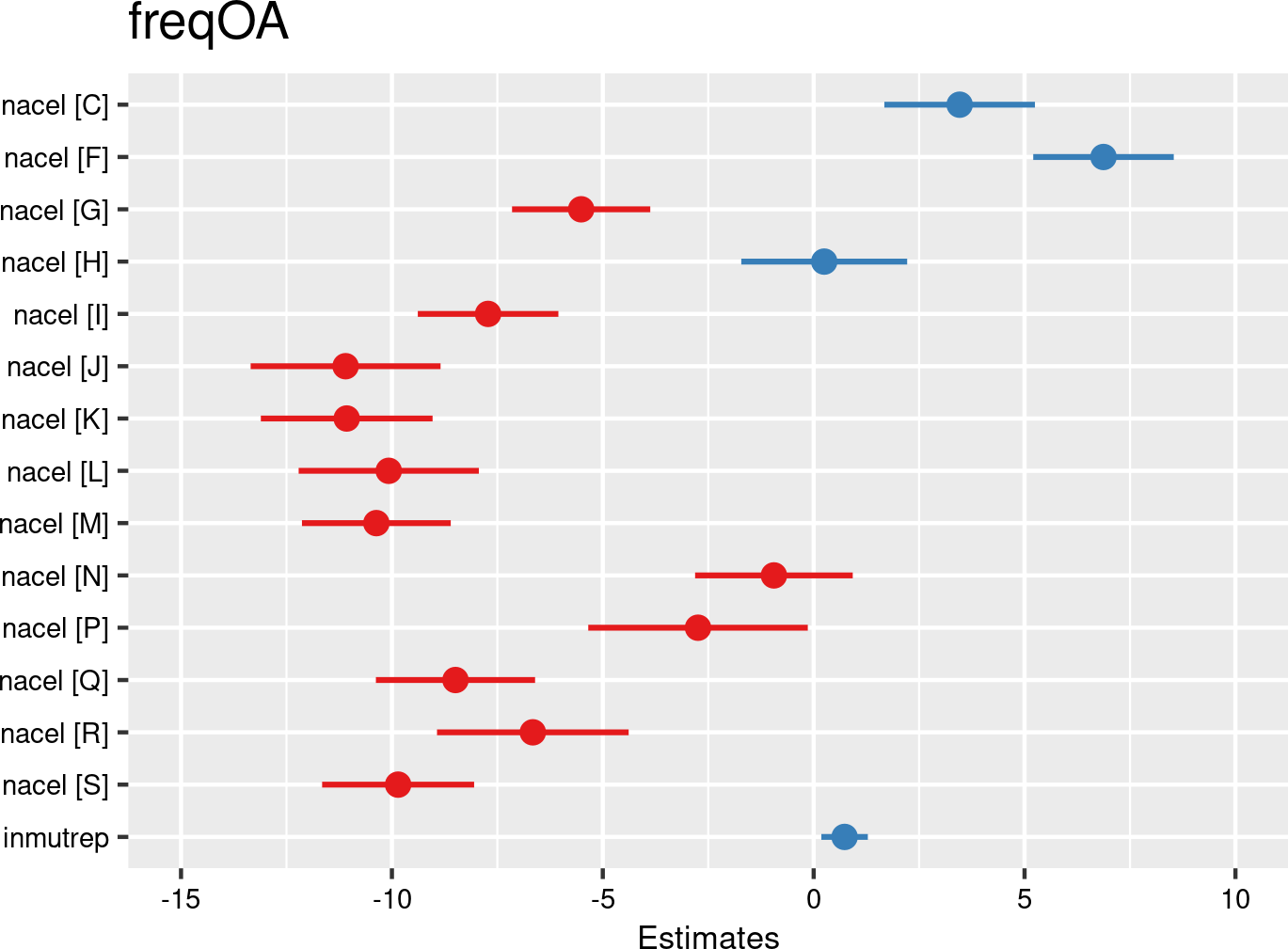

NACE-BEL 2008 Level 1 categories proportions were introduced as fixed effects, and companies as random effects. The model is based on data of all mutual Liantis ESPP and PS customers. The model is adjusted for representativeness of the company (fixed effect inmutrep) regarding to sector, size and Flemish province.
Figure 3.178 (a) and Figure 3.178 (b) present a model estimating the chance for an accepted accident being serious (according to the definition of the Belgian law). These figures indicate that only sector Q (Human health and social work activities) shows significantly lower odds ratios for having an accepted workplace OA classified as serious compared to the reference sector A (Agriculture, forestry and fishing). Other sectors do not show significant differences.
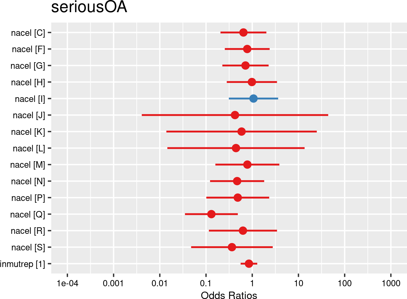

NACE-BEL 2008 Level 1 categories were introduced as fixed effects, and companies and employees as random effects. The model is based on data of all mutual Liantis ESPP and PS customers. The model is adjusted for representativeness of the company (fixed effect inmutrep) regarding to sector, size and Flemish province.
Figure 3.179 (a) and Figure 3.179 (b) show that, compared to the reference sector A (Agriculture, forestry and fishing), sector M (Professional, scientific and technical activities) exhibits significantly lower numbers of (FEDRIS validated) absence days associated with an accepted workplace OA, while sector H (Transportation and storage) shows significantly higher numbers.
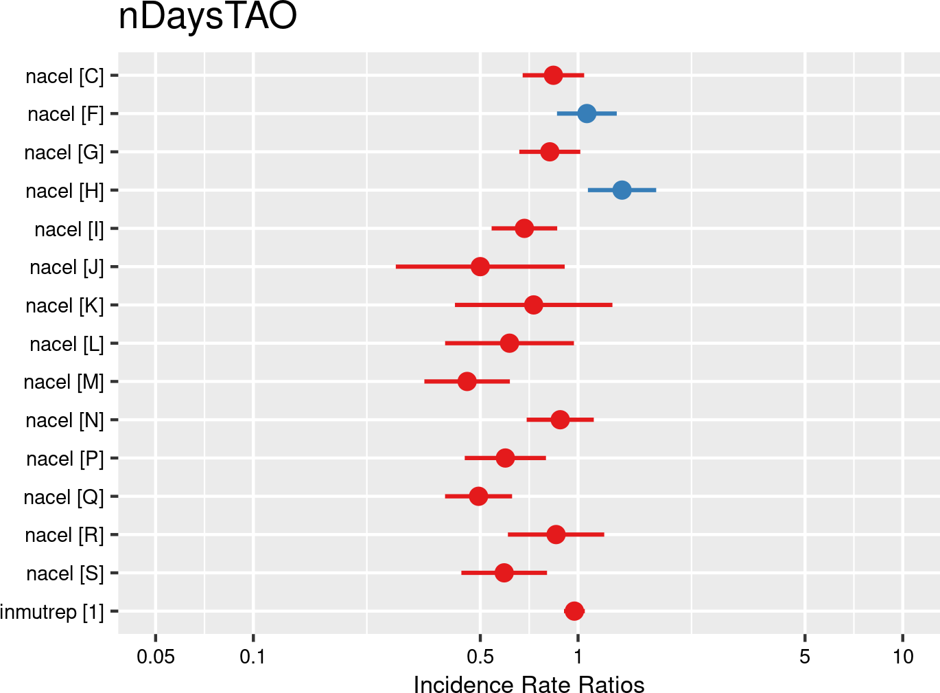

NACE-BEL 2008 Level 1 categories were introduced as fixed effects, and companies and employees as random effects. The model is based on data of all mutual Liantis ESPP and PS customers. The model is adjusted for representativeness of the company (fixed effect inmutrep) regarding to sector, size and Flemish province.
Figure 3.180 (a) and Figure 3.180 (b) largely confirm the results of the previous model with validated days.
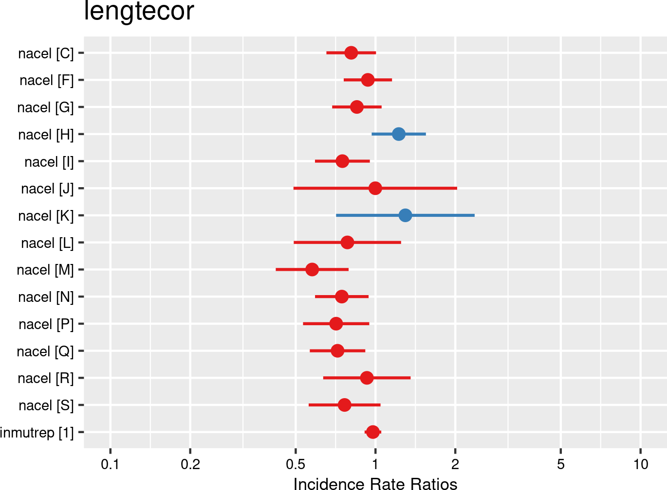

NACE-BEL 2008 Level 1 categories were introduced as fixed effects, and companies and employees as random effects. The model is based on data of all mutual Liantis ESPP and PS customers. The model is adjusted for representativeness of the company (fixed effect inmutrep) regarding to sector, size and Flemish province.
Figure 3.181 (a) and Figure 3.181 (b) show that, compared to the reference sector A (Agriculture, forestry and fishing), sectors C (Manufacturing), F (Construction), H (Transportation and storage) and to a lesser extent N (Administrative and support service activities) exhibit significantly higher direct wage costs associated with an accepted workplace OA, while most other sectors display significantly lower direct wage costs
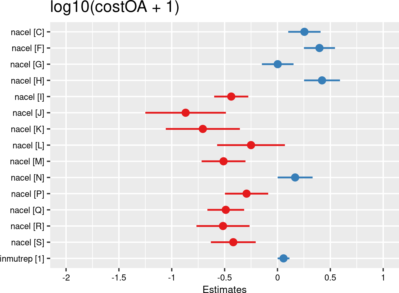

NACE-BEL 2008 Level 1 categories were introduced as fixed effects, and companies and employees as random effects. The model is based on data of all mutual Liantis ESPP and PS customers. The model is adjusted for representativeness of the company (fixed effect inmutrep) regarding to sector, size and Flemish province.
The next 4 figures (Figure 3.182 (a) and Figure 3.182 (b), Figure 3.183 (a) and Figure 3.183 (b)) are displaying the results of models assessing the severity degree of a company in relation to its NACE-BEL 2008 sector. According to Figure 3.182 (a) and Figure 3.182 (b), sector F (Construction) has significantly higher severity degree estimates compared to the reference sector A (Agriculture, forestry and fishing), while most other sectors exhibit significantly lower severity degree estimates
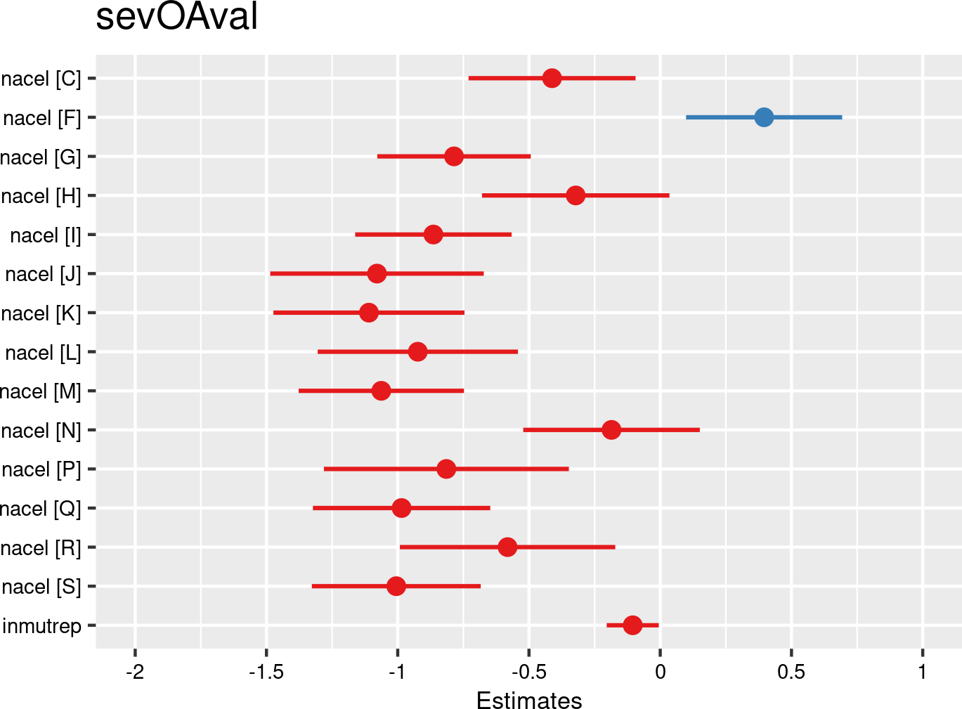

NACE-BEL 2008 Level 1 categories proportions were introduced as fixed effects, and companies as random effects. The model is based on data of all mutual Liantis ESPP and PS customers. The model is adjusted for representativeness of the company (fixed effect inmutrep) regarding to sector, size and Flemish province.
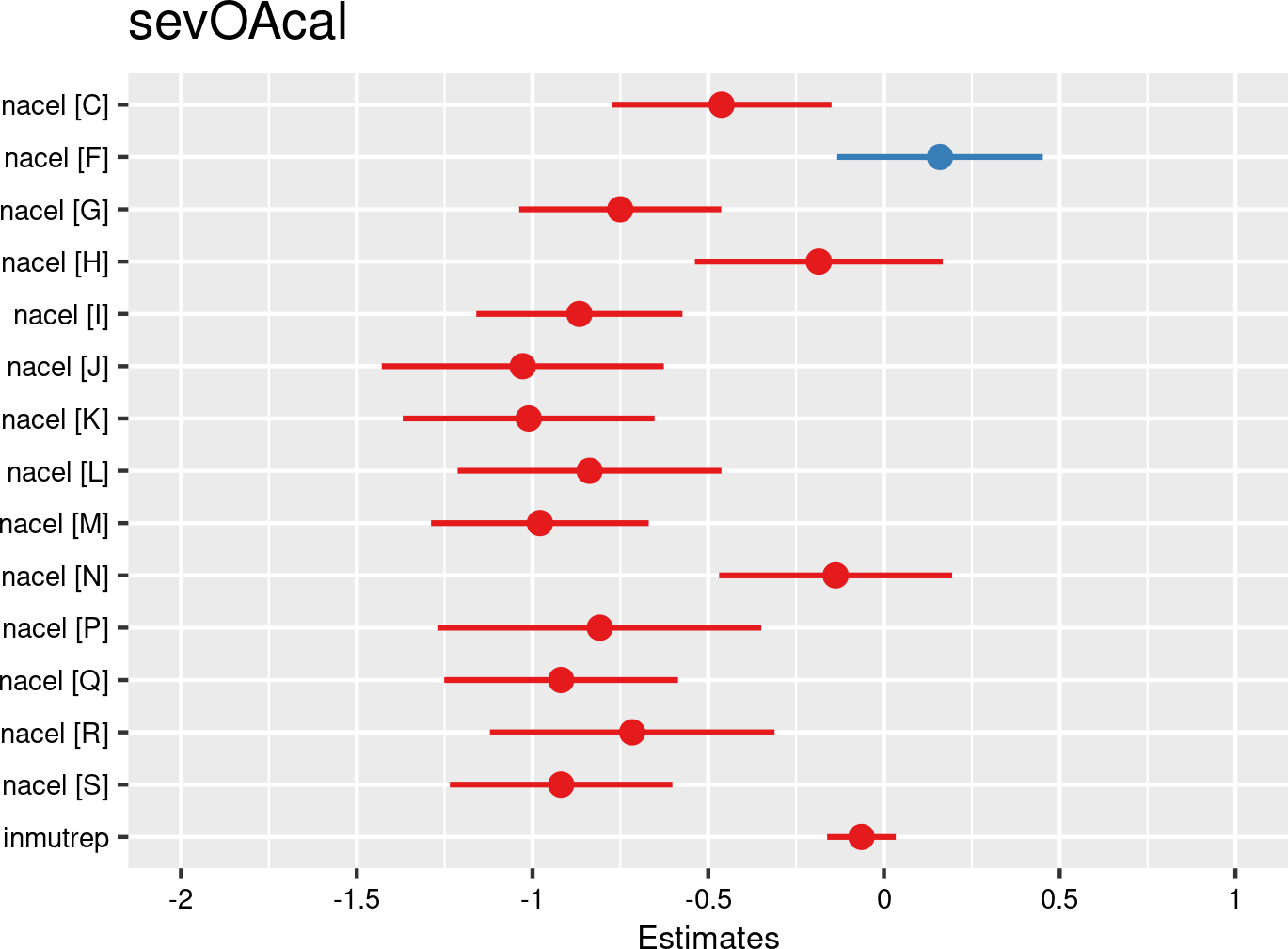

NACE-BEL 2008 Level 1 categories proportions were introduced as fixed effects, and companies as random effects. The model is based on data of all mutual Liantis ESPP and PS customers. The model is adjusted for representativeness of the company (fixed effect inmutrep) regarding to sector, size and Flemish province.
3.4.4.2 Joint labour committees
3.4.4.2.1 Descriptives
Both NSSO and FEDRIS provide statistics on the joint labour committee sector group (in Dutch Paritair Comité (joint collective agreement or sectoral committee) (PC)) of the employee (NSSO 19 groups of joint labour committees, FEDRIS 106 joint labour committees). From Liantis PS data it is also possible to derive the section of the employer through the combined committee and subcommittee codes(6 digits, two times three, first three digits indicate the comittee) of an employer. The notification however does not contain information on the joint labour committee. This information has to be joined from Liantis Payroll data. Since this information is not present in the notification information, the fit between the derived joint labour committee of the employer of an employee experiencing an OA from Liantis data cannot be compared with the corresponding joint labour committee known by NSSO and or FEDRIS and linked to the original notification of the accident.
all accepted occupational accidents
| parcom | rszall | rszpriv | liaall | fedrisall | totalnot | totalnotmut | totalnotrepmutflan |
|---|---|---|---|---|---|---|---|
| Agriculture, horticulture, forestry and sea fishing | 1303435 | 1303435 | 271548 | NA | 954 | 954 | 184 |
| Chemicals and petroleum | 5267391 | 5267391 | 239413 | NA | 391 | 391 | 108 |
| Clothing and textile industry | 1523952 | 1523952 | 177402 | NA | 365 | 365 | 80 |
| Construction | 5713318 | 5713318 | 1100346 | NA | 4631 | 4631 | 1072 |
| Distribution | 10456440 | 10456440 | 1512671 | NA | 2027 | 2027 | 470 |
| Financial sector | 4228631 | 4228631 | 161373 | NA | 73 | 73 | 11 |
| Food industry | 3690570 | 3690570 | 589514 | NA | 2787 | 2787 | 1726 |
| Gas and electricity companies | 702678 | 702678 | 2776 | NA | 3 | 3 | NA |
| Hospitality, sports and recreation | 4782410 | 4782410 | 2766727 | NA | 2192 | 2192 | 312 |
| Media, printing and publishing sector | 573638 | 573638 | 37341 | NA | 38 | 38 | 10 |
| Metal industry | 11225704 | 11225704 | 1135693 | NA | 3768 | 3768 | 1134 |
| Other sectors | 19437471 | 19437471 | 1658501 | NA | 2446 | 2446 | 682 |
| Paper and cardboard industry | 474283 | 474283 | 21256 | NA | 52 | 52 | NA |
| Services to businesses and individuals | 15623907 | 15623907 | 1163038 | NA | 1315 | 1315 | 379 |
| Social profit | 22664565 | 22664565 | 3701139 | NA | 12370 | 12370 | 9594 |
| Stone and glass industry | 668386 | 668386 | 7027 | NA | 5 | 5 | 3 |
| Transport and logistics | 7259434 | 7259434 | 477448 | NA | 1506 | 1506 | 498 |
| Wood industry | 765746 | 765746 | 111925 | NA | 414 | 414 | 94 |
| National Labour Council | NA | NA | NA | NA | 4 | 4 | 2 |
| NA | NA | NA | NA | NA | 159878 | 25894 | 9671 |
| parcom | percrszall | percrszpriv | percliaall | percfedrisall | perctotalnot | perctotalnotmut | perctotalnotrepmutflan |
|---|---|---|---|---|---|---|---|
| Agriculture, horticulture, forestry and sea fishing | 1.1 | 1.1 | 1.8 | NA | 2.7 | 2.7 | 1.1 |
| Chemicals and petroleum | 4.5 | 4.5 | 1.6 | NA | 1.1 | 1.1 | 0.7 |
| Clothing and textile industry | 1.3 | 1.3 | 1.2 | NA | 1.0 | 1.0 | 0.5 |
| Construction | 4.9 | 4.9 | 7.3 | NA | 13.1 | 13.1 | 6.6 |
| Distribution | 9.0 | 9.0 | 10.0 | NA | 5.7 | 5.7 | 2.9 |
| Financial sector | 3.6 | 3.6 | 1.1 | NA | 0.2 | 0.2 | 0.1 |
| Food industry | 3.2 | 3.2 | 3.9 | NA | 7.9 | 7.9 | 10.6 |
| Gas and electricity companies | 0.6 | 0.6 | 0.0 | NA | 0.0 | 0.0 | NA |
| Hospitality, sports and recreation | 4.1 | 4.1 | 18.3 | NA | 6.2 | 6.2 | 1.9 |
| Media, printing and publishing sector | 0.5 | 0.5 | 0.2 | NA | 0.1 | 0.1 | 0.1 |
| Metal industry | 9.6 | 9.6 | 7.5 | NA | 10.7 | 10.7 | 6.9 |
| Other sectors | 16.7 | 16.7 | 11.0 | NA | 6.9 | 6.9 | 4.2 |
| Paper and cardboard industry | 0.4 | 0.4 | 0.1 | NA | 0.1 | 0.1 | NA |
| Services to businesses and individuals | 13.4 | 13.4 | 7.7 | NA | 3.7 | 3.7 | 2.3 |
| Social profit | 19.5 | 19.5 | 24.5 | NA | 35.0 | 35.0 | 58.7 |
| Stone and glass industry | 0.6 | 0.6 | 0.0 | NA | 0.0 | 0.0 | 0.0 |
| Transport and logistics | 6.2 | 6.2 | 3.2 | NA | 4.3 | 4.3 | 3.0 |
| Wood industry | 0.7 | 0.7 | 0.7 | NA | 1.2 | 1.2 | 0.6 |
| National Labour Council | NA | NA | NA | NA | NA | NA | NA |
| NA | NA | NA | NA | NA | NA | NA | NA |
commuting accepted occupational accidents
| parcom | rszall | rszpriv | liaall | fedrisall | totalnot | totalnotmut | totalnotrepmutflan |
|---|---|---|---|---|---|---|---|
| Agriculture, horticulture, forestry and sea fishing | 1303435 | 1303435 | 271548 | NA | 52 | 52 | 12 |
| Chemicals and petroleum | 5267391 | 5267391 | 239413 | NA | 51 | 51 | 18 |
| Clothing and textile industry | 1523952 | 1523952 | 177402 | NA | 47 | 47 | 10 |
| Construction | 5713318 | 5713318 | 1100346 | NA | 223 | 223 | 56 |
| Distribution | 10456440 | 10456440 | 1512671 | NA | 382 | 382 | 92 |
| Financial sector | 4228631 | 4228631 | 161373 | NA | 46 | 46 | 4 |
| Food industry | 3690570 | 3690570 | 589514 | NA | 259 | 259 | 148 |
| Gas and electricity companies | 702678 | 702678 | 2776 | NA | 1 | 1 | NA |
| Hospitality, sports and recreation | 4782410 | 4782410 | 2766727 | NA | 378 | 378 | 50 |
| Media, printing and publishing sector | 573638 | 573638 | 37341 | NA | 12 | 12 | 3 |
| Metal industry | 11225704 | 11225704 | 1135693 | NA | 323 | 323 | 131 |
| Other sectors | 19437471 | 19437471 | 1658501 | NA | 478 | 478 | 170 |
| Paper and cardboard industry | 474283 | 474283 | 21256 | NA | 4 | 4 | NA |
| Services to businesses and individuals | 15623907 | 15623907 | 1163038 | NA | 404 | 404 | 121 |
| Social profit | 22664565 | 22664565 | 3701139 | NA | 2348 | 2348 | 1710 |
| Stone and glass industry | 668386 | 668386 | 7027 | NA | 1 | 1 | NA |
| Transport and logistics | 7259434 | 7259434 | 477448 | NA | 68 | 68 | 28 |
| Wood industry | 765746 | 765746 | 111925 | NA | 40 | 40 | 7 |
| National Labour Council | NA | NA | NA | NA | 1 | 1 | 1 |
| NA | NA | NA | NA | NA | 23269 | 3481 | 1551 |
| parcom | percrszall | percrszpriv | percliaall | percfedrisall | perctotalnot | perctotalnotmut | perctotalnotrepmutflan |
|---|---|---|---|---|---|---|---|
| Agriculture, horticulture, forestry and sea fishing | 1.1 | 1.1 | 1.8 | NA | 1.0 | 1.0 | 0.5 |
| Chemicals and petroleum | 4.5 | 4.5 | 1.6 | NA | 1.0 | 1.0 | 0.7 |
| Clothing and textile industry | 1.3 | 1.3 | 1.2 | NA | 0.9 | 0.9 | 0.4 |
| Construction | 4.9 | 4.9 | 7.3 | NA | 4.4 | 4.4 | 2.2 |
| Distribution | 9.0 | 9.0 | 10.0 | NA | 7.5 | 7.5 | 3.6 |
| Financial sector | 3.6 | 3.6 | 1.1 | NA | 0.9 | 0.9 | 0.2 |
| Food industry | 3.2 | 3.2 | 3.9 | NA | 5.1 | 5.1 | 5.8 |
| Gas and electricity companies | 0.6 | 0.6 | 0.0 | NA | 0.0 | 0.0 | NA |
| Hospitality, sports and recreation | 4.1 | 4.1 | 18.3 | NA | 7.4 | 7.4 | 2.0 |
| Media, printing and publishing sector | 0.5 | 0.5 | 0.2 | NA | 0.2 | 0.2 | 0.1 |
| Metal industry | 9.6 | 9.6 | 7.5 | NA | 6.3 | 6.3 | 5.1 |
| Other sectors | 16.7 | 16.7 | 11.0 | NA | 9.3 | 9.3 | 6.6 |
| Paper and cardboard industry | 0.4 | 0.4 | 0.1 | NA | 0.1 | 0.1 | NA |
| Services to businesses and individuals | 13.4 | 13.4 | 7.7 | NA | 7.9 | 7.9 | 4.7 |
| Social profit | 19.5 | 19.5 | 24.5 | NA | 45.9 | 45.9 | 66.8 |
| Stone and glass industry | 0.6 | 0.6 | 0.0 | NA | 0.0 | 0.0 | NA |
| Transport and logistics | 6.2 | 6.2 | 3.2 | NA | 1.3 | 1.3 | 1.1 |
| Wood industry | 0.7 | 0.7 | 0.7 | NA | 0.8 | 0.8 | 0.3 |
| National Labour Council | NA | NA | NA | NA | NA | NA | NA |
| NA | NA | NA | NA | NA | NA | NA | NA |
workplace accepted occupational accidents
| parcom | rszall | rszpriv | liaall | fedrisall | totalnot | totalnotmut | totalnotrepmutflan |
|---|---|---|---|---|---|---|---|
| Agriculture, horticulture, forestry and sea fishing | 1303435 | 1303435 | 271548 | 14241 | 902 | 902 | 172 |
| Chemicals and petroleum | 5267391 | 5267391 | 239413 | 29552 | 340 | 340 | 90 |
| Clothing and textile industry | 1523952 | 1523952 | 177402 | 16919 | 318 | 318 | 70 |
| Construction | 5713318 | 5713318 | 1100346 | 116241 | 4408 | 4408 | 1016 |
| Distribution | 10456440 | 10456440 | 1512671 | 81235 | 1645 | 1645 | 378 |
| Financial sector | 4228631 | 4228631 | 161373 | 4627 | 27 | 27 | 7 |
| Food industry | 3690570 | 3690570 | 589514 | 44893 | 2528 | 2528 | 1578 |
| Gas and electricity companies | 702678 | 702678 | 2776 | 2333 | 2 | 2 | NA |
| Hospitality, sports and recreation | 4782410 | 4782410 | 2766727 | 34583 | 1814 | 1814 | 262 |
| Media, printing and publishing sector | 573638 | 573638 | 37341 | 3732 | 26 | 26 | 7 |
| Metal industry | 11225704 | 11225704 | 1135693 | 142027 | 3445 | 3445 | 1003 |
| Other sectors | 19437471 | 19437471 | 1658501 | 48430 | 1968 | 1968 | 512 |
| Paper and cardboard industry | 474283 | 474283 | 21256 | 4163 | 48 | 48 | NA |
| Services to businesses and individuals | 15623907 | 15623907 | 1163038 | 160062 | 911 | 911 | 258 |
| Social profit | 22664565 | 22664565 | 3701139 | 215425 | 10022 | 10022 | 7884 |
| Stone and glass industry | 668386 | 668386 | 7027 | 12567 | 4 | 4 | 3 |
| Transport and logistics | 7259434 | 7259434 | 477448 | 76809 | 1438 | 1438 | 470 |
| Wood industry | 765746 | 765746 | 111925 | 12549 | 374 | 374 | 87 |
| National Labour Council | NA | NA | NA | NA | 3 | 3 | 1 |
| NA | NA | NA | NA | NA | 136609 | 22413 | 8120 |
| parcom | percrszall | percrszpriv | percliaall | percfedrisall | perctotalnot | perctotalnotmut | perctotalnotrepmutflan |
|---|---|---|---|---|---|---|---|
| Agriculture, horticulture, forestry and sea fishing | 1.1 | 1.1 | 1.8 | 1.4 | 3.0 | 3.0 | 1.2 |
| Chemicals and petroleum | 4.5 | 4.5 | 1.6 | 2.9 | 1.1 | 1.1 | 0.7 |
| Clothing and textile industry | 1.3 | 1.3 | 1.2 | 1.7 | 1.1 | 1.1 | 0.5 |
| Construction | 4.9 | 4.9 | 7.3 | 11.4 | 14.6 | 14.6 | 7.4 |
| Distribution | 9.0 | 9.0 | 10.0 | 8.0 | 5.4 | 5.4 | 2.7 |
| Financial sector | 3.6 | 3.6 | 1.1 | 0.5 | 0.1 | 0.1 | 0.1 |
| Food industry | 3.2 | 3.2 | 3.9 | 4.4 | 8.4 | 8.4 | 11.4 |
| Gas and electricity companies | 0.6 | 0.6 | 0.0 | 0.2 | 0.0 | 0.0 | NA |
| Hospitality, sports and recreation | 4.1 | 4.1 | 18.3 | 3.4 | 6.0 | 6.0 | 1.9 |
| Media, printing and publishing sector | 0.5 | 0.5 | 0.2 | 0.4 | 0.1 | 0.1 | 0.1 |
| Metal industry | 9.6 | 9.6 | 7.5 | 13.9 | 11.4 | 11.4 | 7.3 |
| Other sectors | 16.7 | 16.7 | 11.0 | 4.7 | 6.5 | 6.5 | 3.7 |
| Paper and cardboard industry | 0.4 | 0.4 | 0.1 | 0.4 | 0.2 | 0.2 | NA |
| Services to businesses and individuals | 13.4 | 13.4 | 7.7 | 15.7 | 3.0 | 3.0 | 1.9 |
| Social profit | 19.5 | 19.5 | 24.5 | 21.1 | 33.2 | 33.2 | 57.1 |
| Stone and glass industry | 0.6 | 0.6 | 0.0 | 1.2 | 0.0 | 0.0 | 0.0 |
| Transport and logistics | 6.2 | 6.2 | 3.2 | 7.5 | 4.8 | 4.8 | 3.4 |
| Wood industry | 0.7 | 0.7 | 0.7 | 1.2 | 1.2 | 1.2 | 0.6 |
| National Labour Council | NA | NA | NA | NA | NA | NA | NA |
| NA | NA | NA | NA | NA | NA | NA | NA |
3.4.4.2.2 Models
The following Table 3.122 table summarizes the results of the models assessing the relationship between the joint labour committees and the several outcomes related to OAs. Below the table, details are provided about the data used for the analyses. The results of the nine models are then presented both graphically and in a table.
| catparcom | chance to notify | chance on refusal | chance commuting | chance workplace | freq degree | chance serious | nDays TAO V/C | cost | sev degree V/C |
|---|---|---|---|---|---|---|---|---|---|
| Agriculture… | REF | REF | REF | REF | REF | REF | REF | REF | REF |
| Chemicals… | < | ns | ns | < | < | ns | ns | ns | </< |
| Clothing… | < | ns | ns | < | < | ns | >/> | > | </< |
| Construction | > | ns | ns | > | > | ns | >/ns | > | ns |
| Distribution | < | ns | ns | < | < | ns | ns | < | </< |
| Financial… | < | ns | ns | < | < | ns | ns | < | </< |
| Food industry | ns | ns | > | < | ns | ns | ns | > | </< |
| Hospitality… | < | ns | ns | < | < | ns | </ns | < | </< |
| Metal industry | ns | ns | ns | ns | ns | ns | ns | > | </< |
| Other sectors | < | ns | ns | < | < | ns | ns | > | </< |
| Paper… | ns | ns | ns | ns | ns | ns | ns | ns | ns |
| Services… | < | ns | > | < | < | ns | ns | ns | </< |
| Social profit | < | ns | > | < | < | < | </ns | < | </< |
| Transport… | < | ns | ns | < | ns | ns | >/> | > | </< |
| Wood industry | ns | ns | > | ns | > | ns | ns | > | ns |
| occur | accept | occur | occur | occur | severe | severe | severe | severe | |
| empl | empl | empl | empl | comp | empl | empl | empl | comp | |
| c/w all | c/w ref | c acc | w acc | w acc | w acc | w acc | w acc | w acc |
- occur: data include all workers, chance for occurrence is calculated for the outcome
- accept: data include only workers with a notification of OA
- severe: data include only workers with an accepted OA
- c/w all: commuting and workplace accidents, including refused and accidents without decisions
- c/w ref: accepted or refused commuting and workplace accidents
- c acc: accepted commuting accidents
- w acc: accepted workplace accidents
- empl: the outcome is situated at the individual level
- comp: the outcome is situated at the company level
- nDaysTAO: number of days absenteeism related to the OA
- V/C: Validated number of days (available from FEDRIS) / Calculated number of days (based on the Liantis PS data)
Joint labour committee and occupational accidents
- Compared to reference joint labour committee Agriculture, horticulture, forestry and sea fishing
- Likelihoods to notify seem to be higher Construction and equal or lower in almost all other committees
- Likelihoods for refusal do not seem to differ significantly between committees
- Likelihoods for experiencing commuting accidents appear to be higher in Food industry and Social profit
- Likelihoods for experiencing workplace accidents appear to be higher in Construction and lower in almost all other sectors (lowest likelihood in the Financial sector)
- Frequency degrees at company level appear to be higher in Construction and Wood industry
- Likelihoods for serious accidents only seems to be lower in Social profit
- Number of absence days associated with an accepted workplace accident seem to be higher in Transport and logistics and Clothing and textile industry and lower in Hospitality, sports and recreation
- Costs appear to be higher in Construction, Transport and logistics and Clothing and textile industry and lower in Financial sector
- Severity degrees at company level appear to be lower in many other committees except Construction
- The influence of joint labour committee as determinant could be further assessed in the multivariable analysis (see Section 3.5) to clarify whether the observed differences persist when adjusting for other variables, but since the correlation between sector (NACE-BEL 2008) and joint labour committee is quite high, multicollinearity issues arise when both variables are included in the same model
From Figure 3.184 (a) and Figure 3.184 (b) we learn that, compared to the reference joint labour committee Agriculture, horticulture, forestry and sea fishing, the committee Construction shows significantly higher odds ratios for notifying an OA, while most other committees exhibit significantly lower odds ratios.
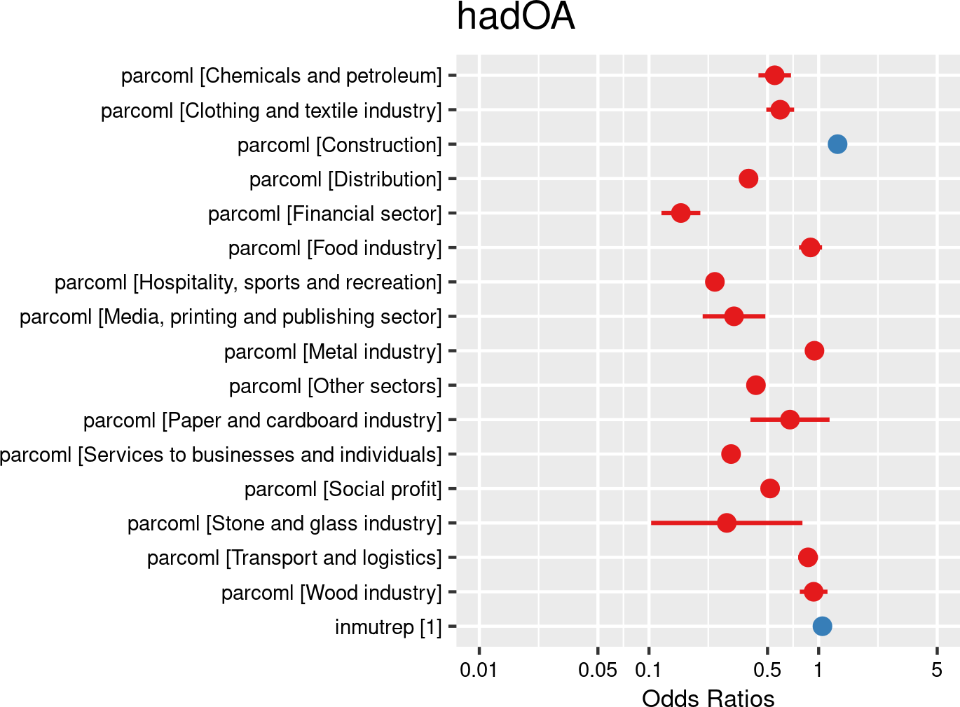

Joint labour committee categories were introduced as fixed effects, and companies and employees as random effects. The model is based on data of a sample of 50,000 workers. The model is adjusted for representativeness of the company (fixed effect inmutrep) regarding to sector, size and Flemish province.
According to Figure 3.185 (a) and Figure 3.185 (b), the joint labour committee of a company is not significantly associated with the odds of having a reported OA being refused by the insurer.
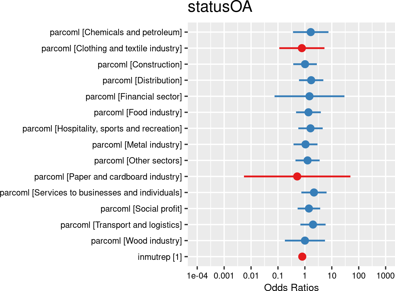

Joint labour committee categories were introduced as fixed effects, and companies and employees as random effects. The model is based on data of all employees. The model is adjusted for representativeness of the company (fixed effect inmutrep) regarding to sector, size and Flemish province.
According to Figure 3.186 (a) and Figure 3.186 (b), the likelihoods for experiencing commuting accidents appear to be higher in Food industry, Social profit and Services to businesses and individuals compared to the reference joint labour committee Agriculture, horticulture, forestry and sea fishing.
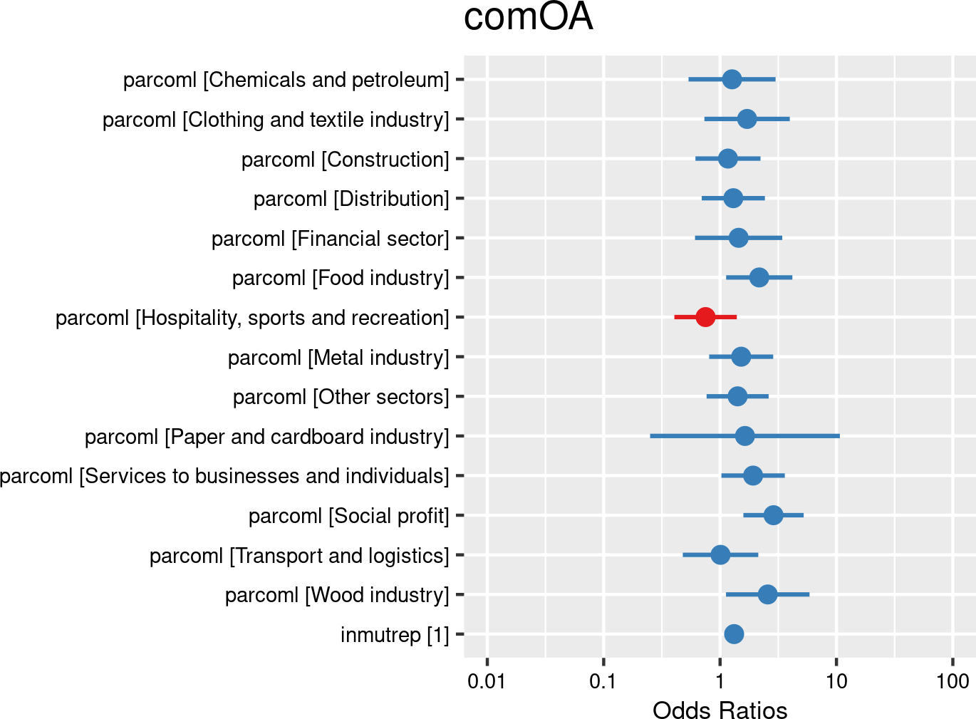

Joint labour committee categories were introduced as fixed effects, and companies and employees as random effects. The model is based on data of a sample of 50.000 workers. The model is adjusted for representativeness of the company (fixed effect inmutrep) regarding to sector, size and Flemish province.
Figure 3.187 (a) and Figure 3.187 (b) show that, compared to the reference joint labour committee Agriculture, horticulture, forestry and sea fishing, the committee Construction exhibits significantly higher odds ratios for accepted workplace accidents, while most other committees display significantly lower odds ratios.
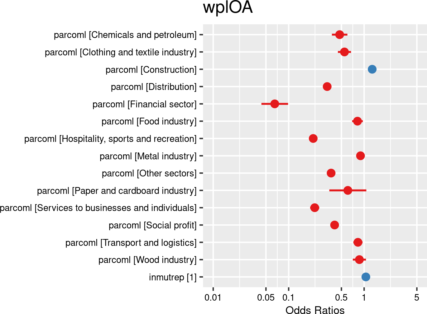

Joint labour committee categories were introduced as fixed effects, and companies and employees as random effects. The model is based on data of a sample of 50.000 workers. The model is adjusted for representativeness of the company (fixed effect inmutrep) regarding to sector, size and Flemish province.
Figure 3.188 (a) and Figure 3.188 (b) present a model estimating the frequency degree of OA at the company level. These figures indicate that the committee Construction and Wood industry have significantly higher frequency degree estimates compared to the reference joint labour committee Agriculture, horticulture, forestry and sea fishing.
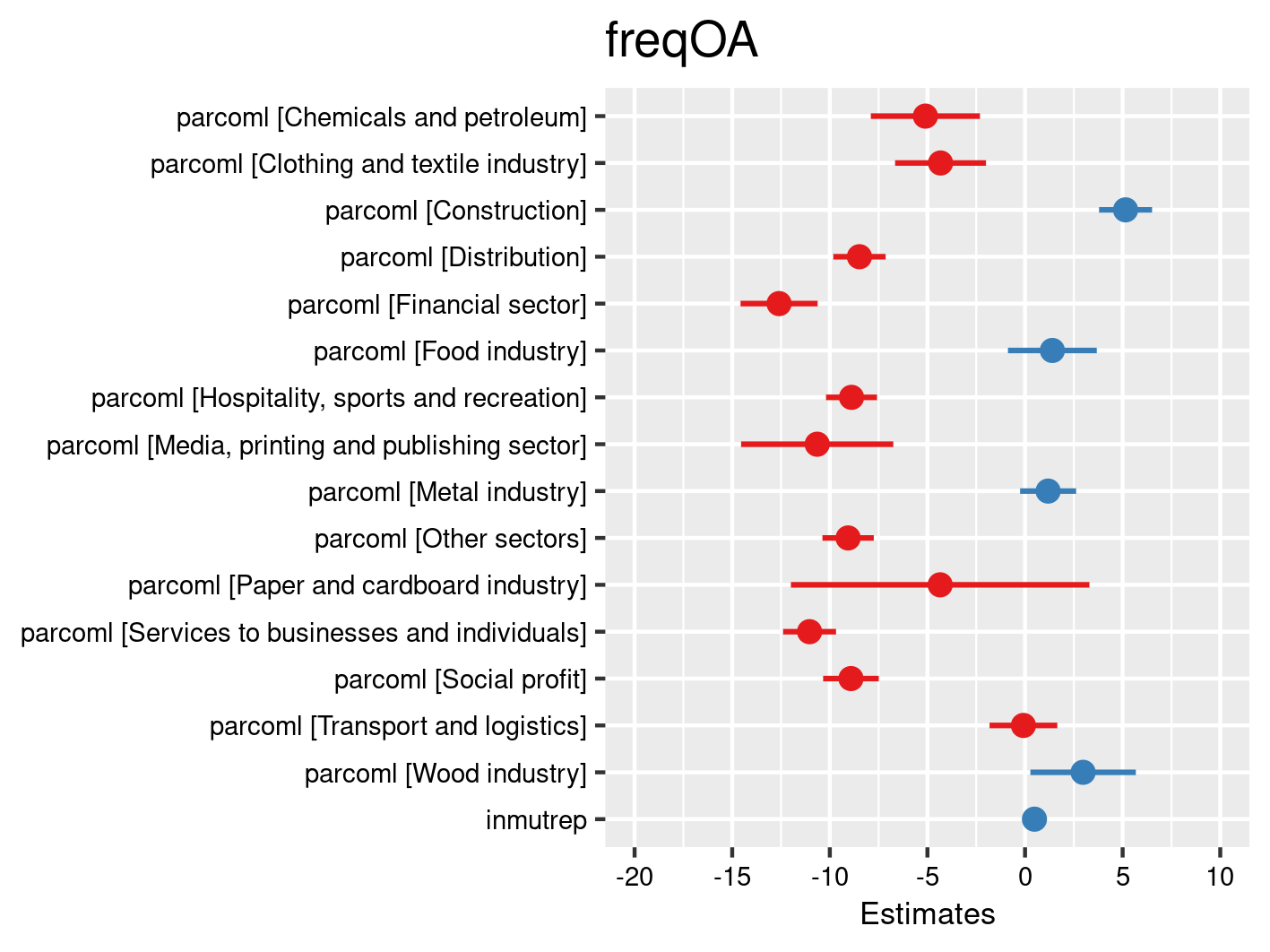

Joint labour committee categories proportions were introduced as fixed effects, and companies as random effects. The model is based on data of all mutual Liantis ESPP and PS customers. The model is adjusted for representativeness of the company (fixed effect inmutrep) regarding to sector, size and Flemish province.
Figure 3.189 (a) and Figure 3.189 (b) present a model estimating the chance for an accepted accident being serious (according to the definition of the Belgian law). These figures indicate that only committee Social profit shows significantly lower odds ratios for having an accepted workplace OA classified as serious compared to the reference joint labour committee Agriculture, horticulture, forestry and sea fishing. Other committees do not show significant differences.
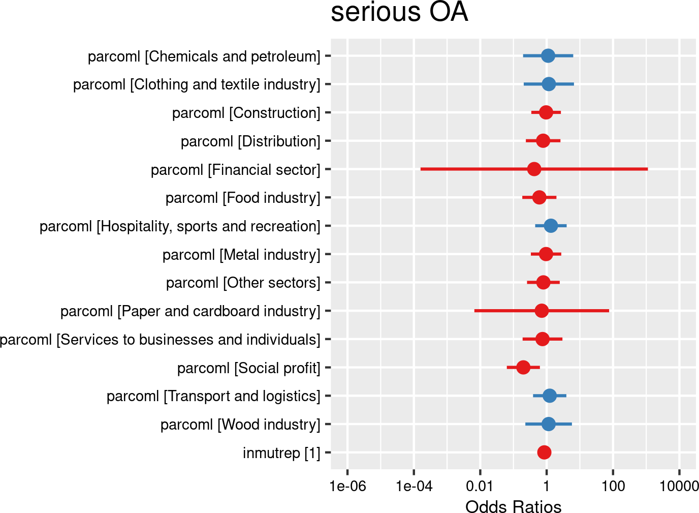

Joint labour committee categories were introduced as fixed effects, and companies and employees as random effects. The model is based on data of all mutual Liantis ESPP and PS customers. The model is adjusted for representativeness of the company (fixed effect inmutrep) regarding to sector, size and Flemish province.
Figure 3.190 (a) and Figure 3.190 (b) show that, compared to the reference joint labour committee Agriculture, horticulture, forestry and sea fishing, committee Transport and logistics and Clothing and textile industry exhibit significantly higher numbers of (FEDRIS validated) absence days associated with an accepted workplace OA, while committee Hospitality, sports and recreation and Social profit show significantly lower numbers.
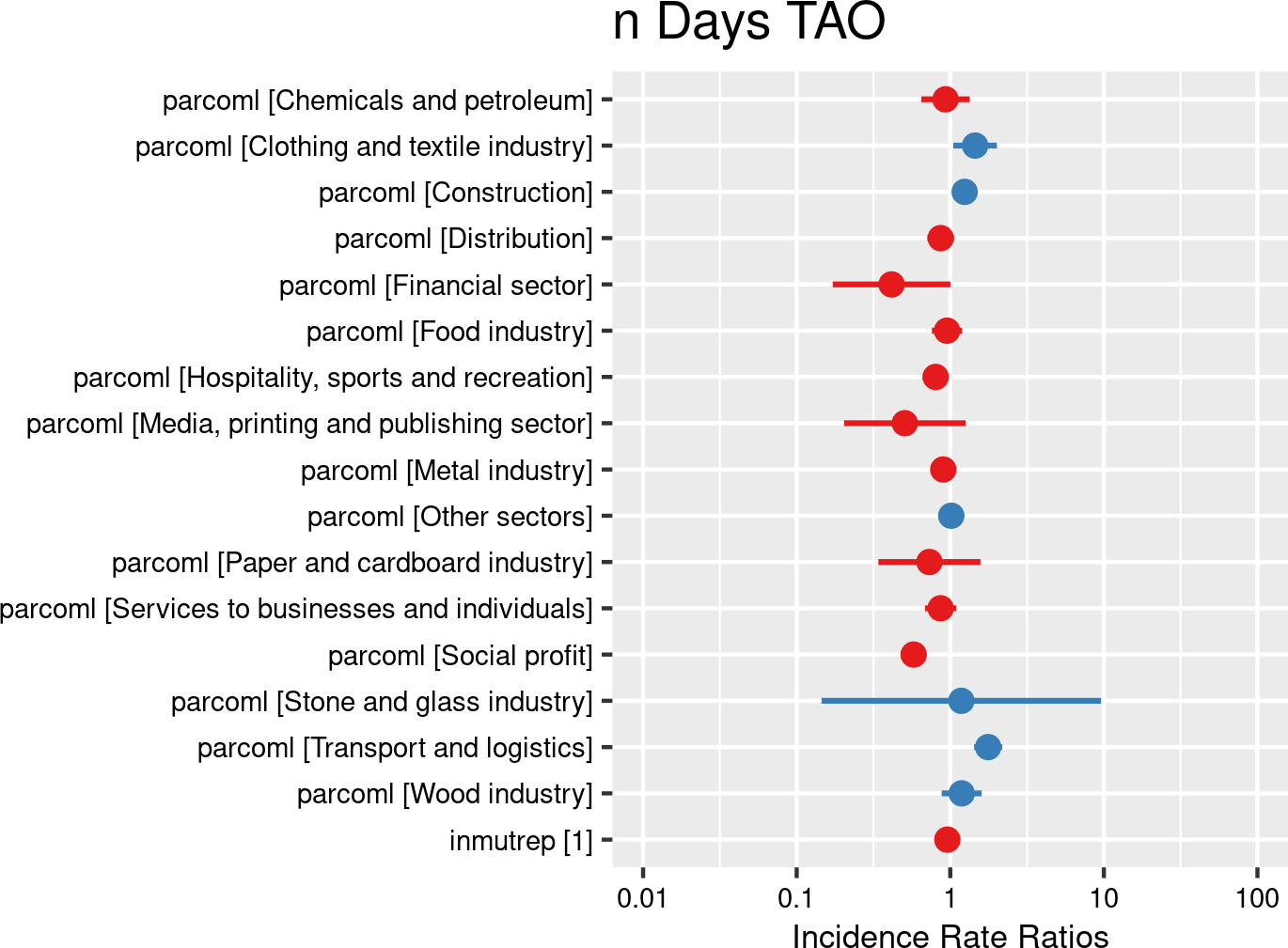

Joint labour committee categories were introduced as fixed effects, and companies and employees as random effects. The model is based on data of all mutual Liantis ESPP and PS customers. The model is adjusted for representativeness of the company (fixed effect inmutrep) regarding to sector, size and Flemish province.
Figure 3.191 (a) and Figure 3.191 (b) confirm the results of the previous model with validated days for Clothing and textile industry and Transport and logistics.
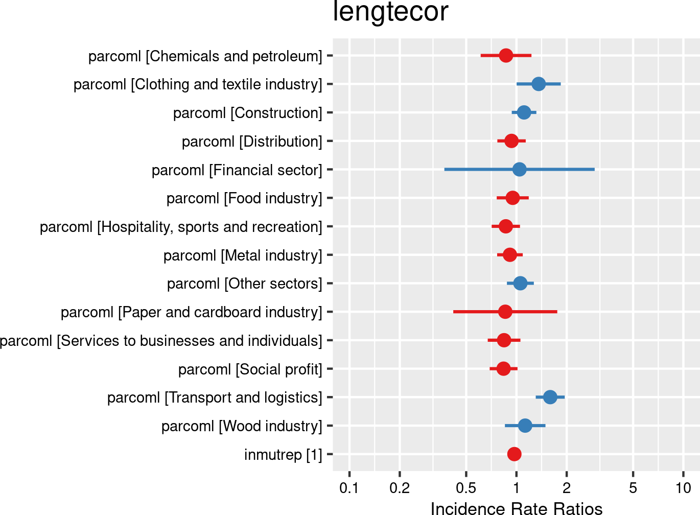

Joint labour committee categories were introduced as fixed effects, and companies and employees as random effects. The model is based on data of all mutual Liantis ESPP and PS customers. The model is adjusted for representativeness of the company (fixed effect inmutrep) regarding to sector, size and Flemish province.
Figure 3.192 (a) and Figure 3.192 (b) show that, compared to the reference joint labour committee Agriculture, horticulture, forestry and sea fishing, committees Construction, Transport and logistics and Clothing and textile industry exhibit significantly higher direct wage costs associated with an accepted workplace OA, while Financial sector and social profit display significantly lower direct wage costs.
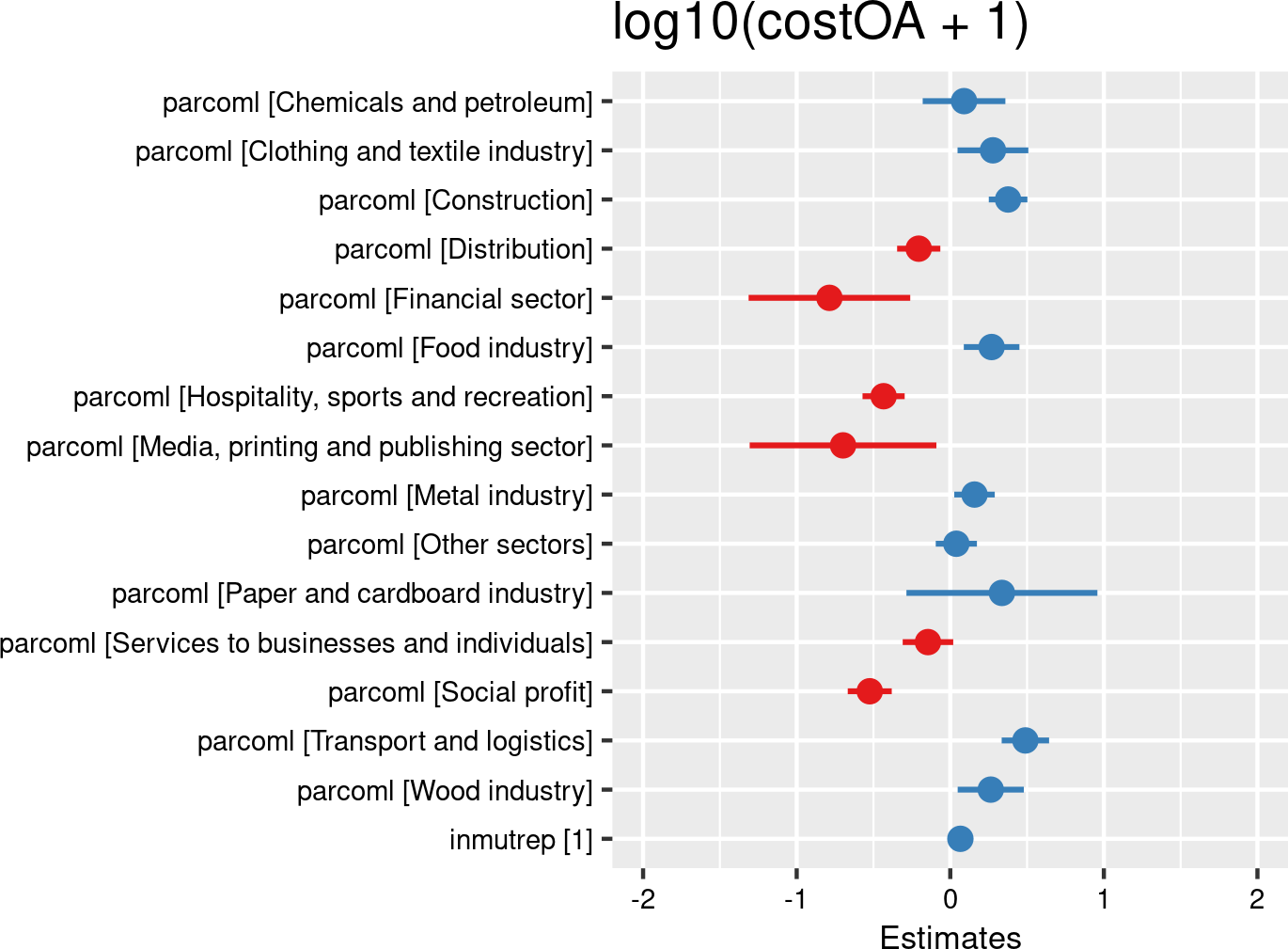

Joint labour committee categories were introduced as fixed effects, and companies and employees as random effects. The model is based on data of all mutual Liantis ESPP and PS customers. The model is adjusted for representativeness of the company (fixed effect inmutrep) regarding to sector, size and Flemish province.
The next 4 figures (Figure 3.193 (a) and Figure 3.193 (b), Figure 3.194 (a) and Figure 3.194 (b)) are displaying the results of models assessing the severity degree of a company in relation to its joint labour committee. According to Figure 3.193 (a) and Figure 3.193 (b), committee Construction has significantly higher severity degree estimates compared to the reference joint labour committee Agriculture, horticulture, forestry and sea fishing, while most other committees exhibit significantly lower severity degree estimates
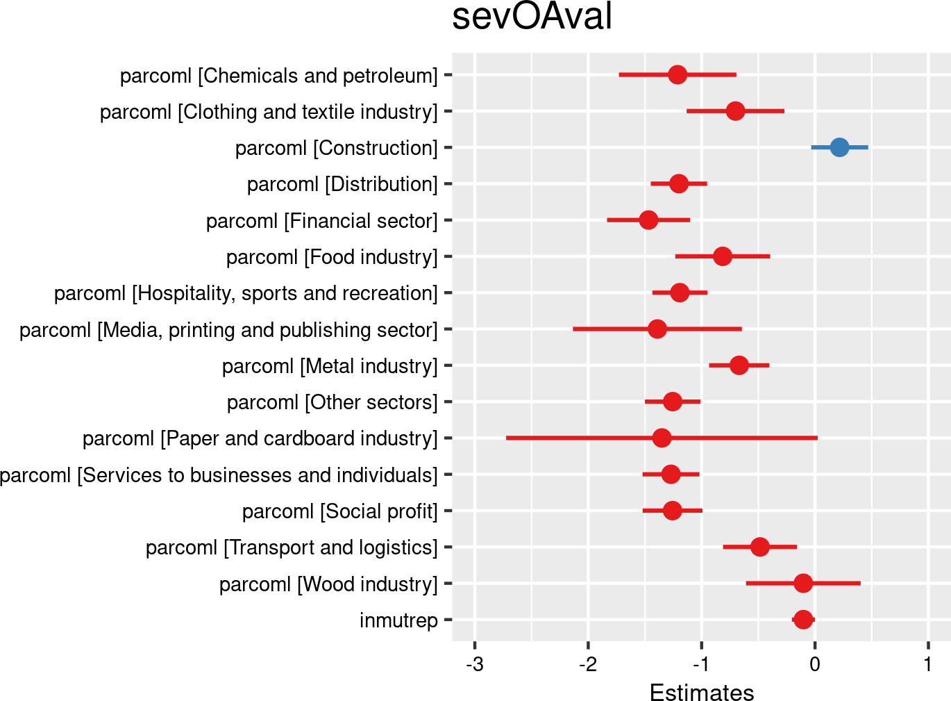

Joint labour committee categories proportions were introduced as fixed effects, and companies as random effects. The model is based on data of all mutual Liantis ESPP and PS customers. The model is adjusted for representativeness of the company (fixed effect inmutrep) regarding to sector, size and Flemish province.
The model below Figure 3.194 (a) and Figure 3.194 (b) largely confirms the results of the previous model with validated days.
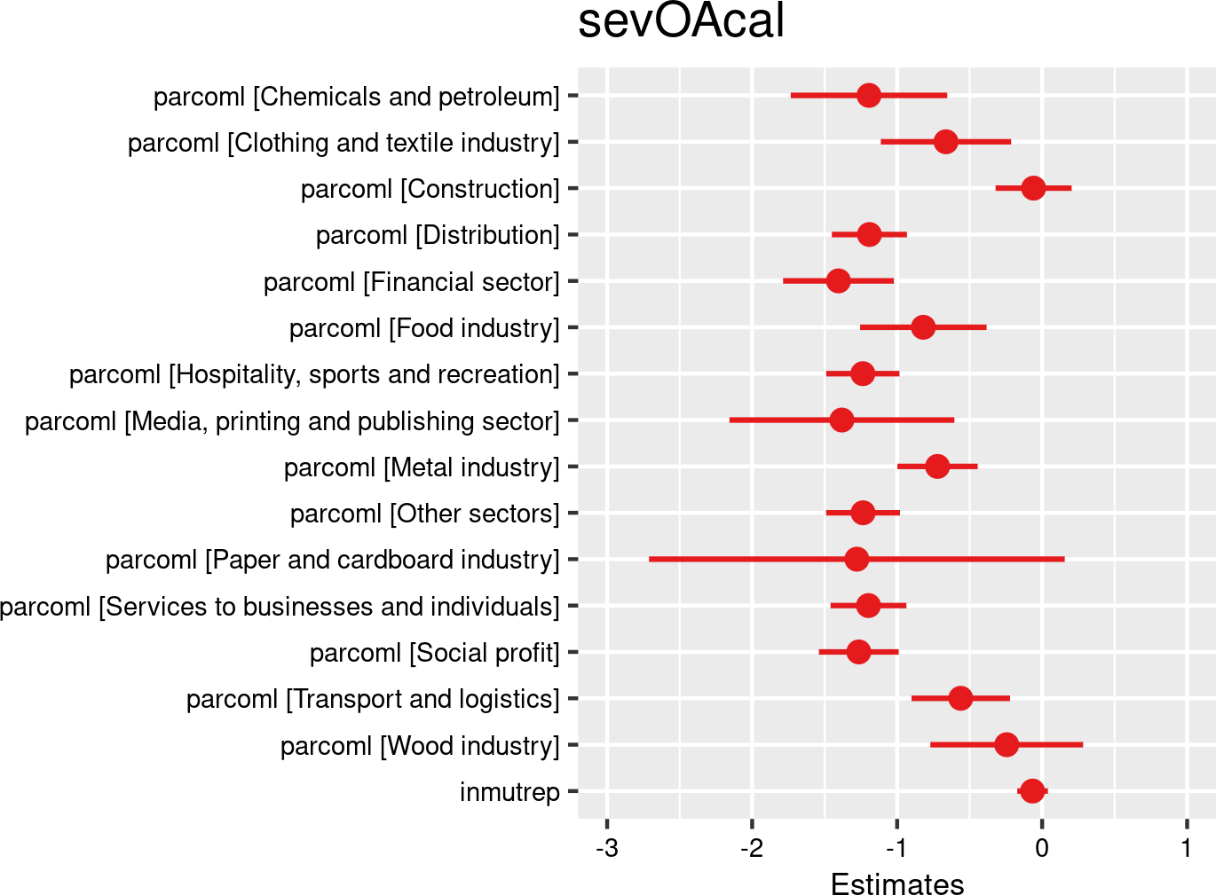

Joint labour committee categories proportions were introduced as fixed effects, and companies as random effects. The model is based on data of all mutual Liantis ESPP and PS customers. The model is adjusted for representativeness of the company (fixed effect inmutrep) regarding to sector, size and Flemish province.
3.4.5 Temporal patterns
3.4.5.1 Time trend (years)
3.4.5.1.1 Descriptives
Both NSSO and FEDRIS provide yearly statistics with counts of employees and employers. The same counts can be made for Liantis PS data. The notification contains the date (and thus year) of the OA.
all accepted occupational accidents
| year | rszall | rszpriv | liaall | fedrisall | totalnot | totalnotmut | totalnotrepmutflan |
|---|---|---|---|---|---|---|---|
| 2014 | 13618344 | 10818747 | 1421509 | 141865 | 18309 | 5736 | 2287 |
| 2015 | 13726629 | 10926121 | 1516903 | 137219 | 18205 | 5729 | 2350 |
| 2016 | 13885634 | 11087143 | 1545854 | 142229 | 19289 | 6212 | 2551 |
| 2017 | 15495893 | 11256351 | 1644027 | 145538 | 19547 | 6475 | 2680 |
| 2018 | 15686057 | 11433166 | 1730173 | 147124 | 21901 | 6315 | 2608 |
| 2019 | 15916663 | 11619292 | 1828135 | 146507 | 22074 | 6423 | 2752 |
| 2020 | 15858180 | 11536574 | 1832210 | 114086 | 18120 | 5414 | 2346 |
| 2021 | 16115691 | 11741334 | 1948030 | 125946 | 19403 | 6110 | 2648 |
| 2022 | 16385592 | 11977770 | 2169919 | 127296 | 19170 | 6422 | 2848 |
| 2023 | 16479459 | 12038328 | 2419106 | 125567 | 19201 | 6399 | 2960 |
| year | percrszall | percrszpriv | percliaall | percfedrisall | perctotalnot | perctotalnotmut | perctotalnotrepmutflan |
|---|---|---|---|---|---|---|---|
| 2014 | 8.89 | 9.45 | 7.87 | 10.48 | 9.38 | 9.37 | 8.79 |
| 2015 | 8.96 | 9.55 | 8.40 | 10.14 | 9.33 | 9.36 | 9.03 |
| 2016 | 9.07 | 9.69 | 8.56 | 10.51 | 9.88 | 10.14 | 9.80 |
| 2017 | 10.12 | 9.84 | 9.11 | 10.75 | 10.01 | 10.57 | 10.30 |
| 2018 | 10.24 | 9.99 | 9.58 | 10.87 | 11.22 | 10.31 | 10.02 |
| 2019 | 10.39 | 10.15 | 10.12 | 10.83 | 11.31 | 10.49 | 10.57 |
| 2020 | 10.35 | 10.08 | 10.15 | 8.43 | 9.28 | 8.84 | 9.01 |
| 2021 | 10.52 | 10.26 | 10.79 | 9.31 | 9.94 | 9.98 | 10.17 |
| 2022 | 10.70 | 10.47 | 12.02 | 9.41 | 9.82 | 10.49 | 10.94 |
| 2023 | 10.76 | 10.52 | 13.40 | 9.28 | 9.84 | 10.45 | 11.37 |
commuting accepted occupational accidents
| year | rszall | rszpriv | liaall | fedrisall | totalnot | totalnotmut | totalnotrepmutflan |
|---|---|---|---|---|---|---|---|
| 2014 | 13618344 | 10818747 | 1421509 | 20670 | 2228 | 668 | 298 |
| 2015 | 13726629 | 10926121 | 1516903 | 20772 | 2424 | 761 | 333 |
| 2016 | 13885634 | 11087143 | 1545854 | 22347 | 2562 | 759 | 347 |
| 2017 | 15495893 | 11256351 | 1644027 | 24627 | 2945 | 960 | 431 |
| 2018 | 15686057 | 11433166 | 1730173 | 24389 | 3102 | 797 | 356 |
| 2019 | 15916663 | 11619292 | 1828135 | 26429 | 3408 | 935 | 426 |
| 2020 | 15858180 | 11536574 | 1832210 | 17920 | 2504 | 708 | 351 |
| 2021 | 16115691 | 11741334 | 1948030 | 20660 | 2879 | 863 | 451 |
| 2022 | 16385592 | 11977770 | 2169919 | 23726 | 3111 | 1047 | 516 |
| 2023 | 16479459 | 12038328 | 2419106 | 24770 | 3224 | 1101 | 603 |
| year | percrszall | percrszpriv | percliaall | percfedrisall | perctotalnot | perctotalnotmut | perctotalnotrepmutflan |
|---|---|---|---|---|---|---|---|
| 2014 | 8.89 | 9.45 | 7.87 | 9.13 | 7.85 | 7.77 | 7.25 |
| 2015 | 8.96 | 9.55 | 8.40 | 9.18 | 8.54 | 8.85 | 8.10 |
| 2016 | 9.07 | 9.69 | 8.56 | 9.87 | 9.03 | 8.83 | 8.44 |
| 2017 | 10.12 | 9.84 | 9.11 | 10.88 | 10.37 | 11.16 | 10.48 |
| 2018 | 10.24 | 9.99 | 9.58 | 10.78 | 10.93 | 9.27 | 8.66 |
| 2019 | 10.39 | 10.15 | 10.12 | 11.68 | 12.01 | 10.87 | 10.36 |
| 2020 | 10.35 | 10.08 | 10.15 | 7.92 | 8.82 | 8.23 | 8.54 |
| 2021 | 10.52 | 10.26 | 10.79 | 9.13 | 10.14 | 10.04 | 10.97 |
| 2022 | 10.70 | 10.47 | 12.02 | 10.48 | 10.96 | 12.18 | 12.55 |
| 2023 | 10.76 | 10.52 | 13.40 | 10.95 | 11.36 | 12.80 | 14.66 |
workplace accepted occupational accidents
| year | rszall | rszpriv | liaall | fedrisall | totalnot | totalnotmut | totalnotrepmutflan |
|---|---|---|---|---|---|---|---|
| 2014 | 13618344 | 10818747 | 1421509 | 121195 | 16081 | 5068 | 1989 |
| 2015 | 13726629 | 10926121 | 1516903 | 116447 | 15781 | 4968 | 2017 |
| 2016 | 13885634 | 11087143 | 1545854 | 119882 | 16727 | 5453 | 2204 |
| 2017 | 15495893 | 11256351 | 1644027 | 120911 | 16602 | 5515 | 2249 |
| 2018 | 15686057 | 11433166 | 1730173 | 122735 | 18799 | 5518 | 2252 |
| 2019 | 15916663 | 11619292 | 1828135 | 120078 | 18666 | 5488 | 2326 |
| 2020 | 15858180 | 11536574 | 1832210 | 96166 | 15616 | 4706 | 1995 |
| 2021 | 16115691 | 11741334 | 1948030 | 105286 | 16524 | 5247 | 2197 |
| 2022 | 16385592 | 11977770 | 2169919 | 103570 | 16059 | 5375 | 2332 |
| 2023 | 16479459 | 12038328 | 2419106 | 100797 | 15977 | 5298 | 2357 |
| year | percrszall | percrszpriv | percliaall | percfedrisall | perctotalnot | perctotalnotmut | perctotalnotrepmutflan |
|---|---|---|---|---|---|---|---|
| 2014 | 8.89 | 9.45 | 7.87 | 10.75 | 9.64 | 9.63 | 9.07 |
| 2015 | 8.96 | 9.55 | 8.40 | 10.33 | 9.46 | 9.44 | 9.20 |
| 2016 | 9.07 | 9.69 | 8.56 | 10.64 | 10.03 | 10.36 | 10.06 |
| 2017 | 10.12 | 9.84 | 9.11 | 10.73 | 9.95 | 10.48 | 10.26 |
| 2018 | 10.24 | 9.99 | 9.58 | 10.89 | 11.27 | 10.48 | 10.27 |
| 2019 | 10.39 | 10.15 | 10.12 | 10.65 | 11.19 | 10.43 | 10.61 |
| 2020 | 10.35 | 10.08 | 10.15 | 8.53 | 9.36 | 8.94 | 9.10 |
| 2021 | 10.52 | 10.26 | 10.79 | 9.34 | 9.90 | 9.97 | 10.02 |
| 2022 | 10.70 | 10.47 | 12.02 | 9.19 | 9.63 | 10.21 | 10.64 |
| 2023 | 10.76 | 10.52 | 13.40 | 8.94 | 9.58 | 10.07 | 10.75 |
3.4.5.1.2 Models
The following Table 3.129 table summarizes the results of the models assessing the relationship between the different years of the study and the several outcomes related to OAs. Below the table, details are provided about the data used for the analyses. The results of the nine models are then presented both graphically and in a table.
| catyear | chance to notify | chance on refusal | chance commuting | chance workplace | freq degree | chance serious | nDays TAO V/C | cost | sev degree V/C |
|---|---|---|---|---|---|---|---|---|---|
| 2014 | REF | REF | REF | REF | REF | REF | REF | REF | REF |
| 2015 | < | ns | ns | < | < | ns | ns/ns | > | ns |
| 2016 | ns | ns | ns | ns | < | ns | >/ns | > | ns |
| 2017 | ns | ns | > | ns | < | ns | ns/ns | > | ns |
| 2018 | < | ns | ns | < | < | ns | ns/ns | > | ns |
| 2019 | < | ns | ns | < | < | ns | >/> | > | ns |
| 2020 | < | ns | < | < | < | > | >/ns | > | ns/< |
| 2021 | < | ns | ns | < | < | ns | >/> | > | ns/< |
| 2022 | < | > | ns | < | < | ns | >/> | > | ns/< |
| 2023 | < | > | ns | < | < | > | ns/ns | > | </< |
| occur | accept | occur | occur | occur | severe | severe | severe | severe | |
| empl | empl | empl | empl | comp | empl | empl | empl | comp | |
| c/w all | c/w ref | c acc | w acc | w acc | w acc | w acc | w acc | w acc |
- occur: data include all workers, chance for occurrence is calculated for the outcome
- accept: data include only workers with a notification of OA
- severe: data include only workers with an accepted OA
- c/w all: commuting and workplace accidents, including refused and accidents without decisions
- c/w ref: accepted or refused commuting and workplace accidents
- c acc: accepted commuting accidents
- w acc: accepted workplace accidents
- empl: the outcome is situated at the individual level
- comp: the outcome is situated at the company level
- nDaysTAO: number of days absenteeism related to the OA
- V/C: Validated number of days (available from FEDRIS) / Calculated number of days (based on the Liantis PS data)
Time trend (years) and occupational accidents
- Compared to reference year 2014, the likelihoods to notify were significantly lower in almost all years except 2016 and 2017
- The likelihoods for refusal were significantly higher in 2022 and 2023
- The likelihoods for experiencing commuting occupational accidents were significantly lower in 2020, but significantly higher in 2017
- The likelihoods for experiencing workplace occupational accidents were significantly lower in almost all years with exception of 2016; a general decreasing trend in odds ratios is observed over the years
- The same decreasing trend is observed for the frequency degree estimates at company level
- The likelihoods for experiencing serious accidents were significantly higher in 2020 and 2023
- The numbers of absence days associated with an accepted workplace OA were significantly higher in 2021 and 2022
- Estimates of cost related to occupational accidents were significantly higher for all years and, with exception of 2018, seemed to be gradually increasing up tot 2021
- The severity degree estimates at company level were significantly lower in 2023 (validated) and in 2020 to 2023 (calculated), a decreasing trend -however less clear than for the frequency degrees- can be noticed
From Figure 3.195 (a) and Figure 3.195 (b) we learn that, compared to the reference year 2014, the likelihoods to notify were significantly lower in almost all years except 2016 and 2017.
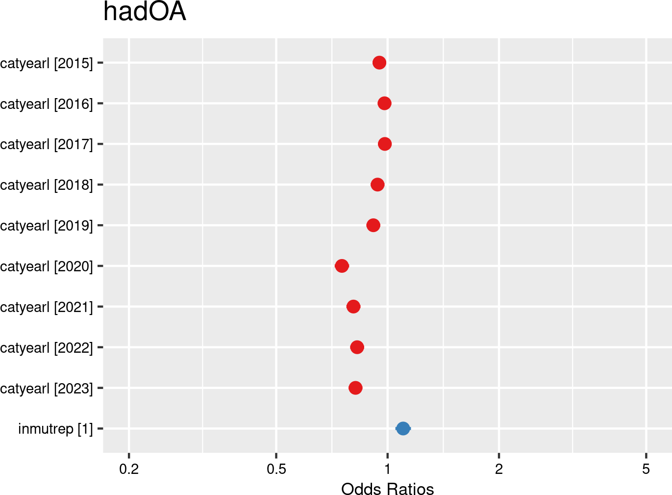

Years were introduced as fixed effects, and companies and employees as random effects. The model is based on data of a sample of 50,000 workers. The model is adjusted for representativeness of the company (fixed effect inmutrep) regarding to sector, size and Flemish province.
According to Figure 3.196 (a) and Figure 3.196 (b), the likelihoods for refusal were significantly higher in 2022 and 2023 compared to the reference year 2014.
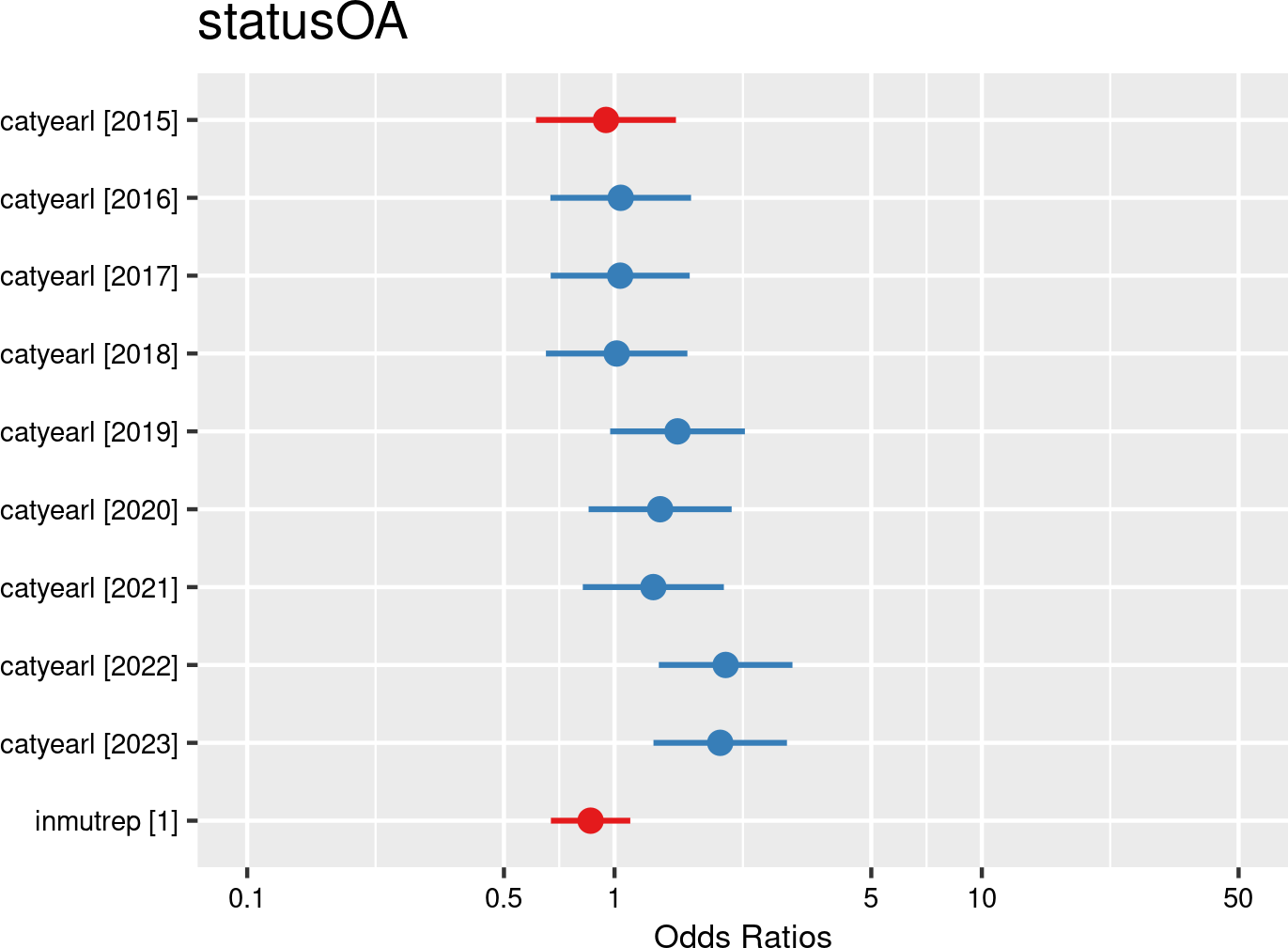

Years were introduced as fixed effects, and companies and employees as random effects. The model is based on data of all employees. The model is adjusted for representativeness of the company (fixed effect inmutrep) regarding to sector, size and Flemish province.
According to Figure 3.197 (a) and Figure 3.197 (b), the likelihoods for experiencing commuting occupational accidents were significantly lower in 2020, but significantly higher in 2017 compared to the reference year 2014. The steep drop in 2020 can likely be attributed to the COVID-19 pandemic and associated lockdowns, which reduced commuting activities (see Figure 2.61).
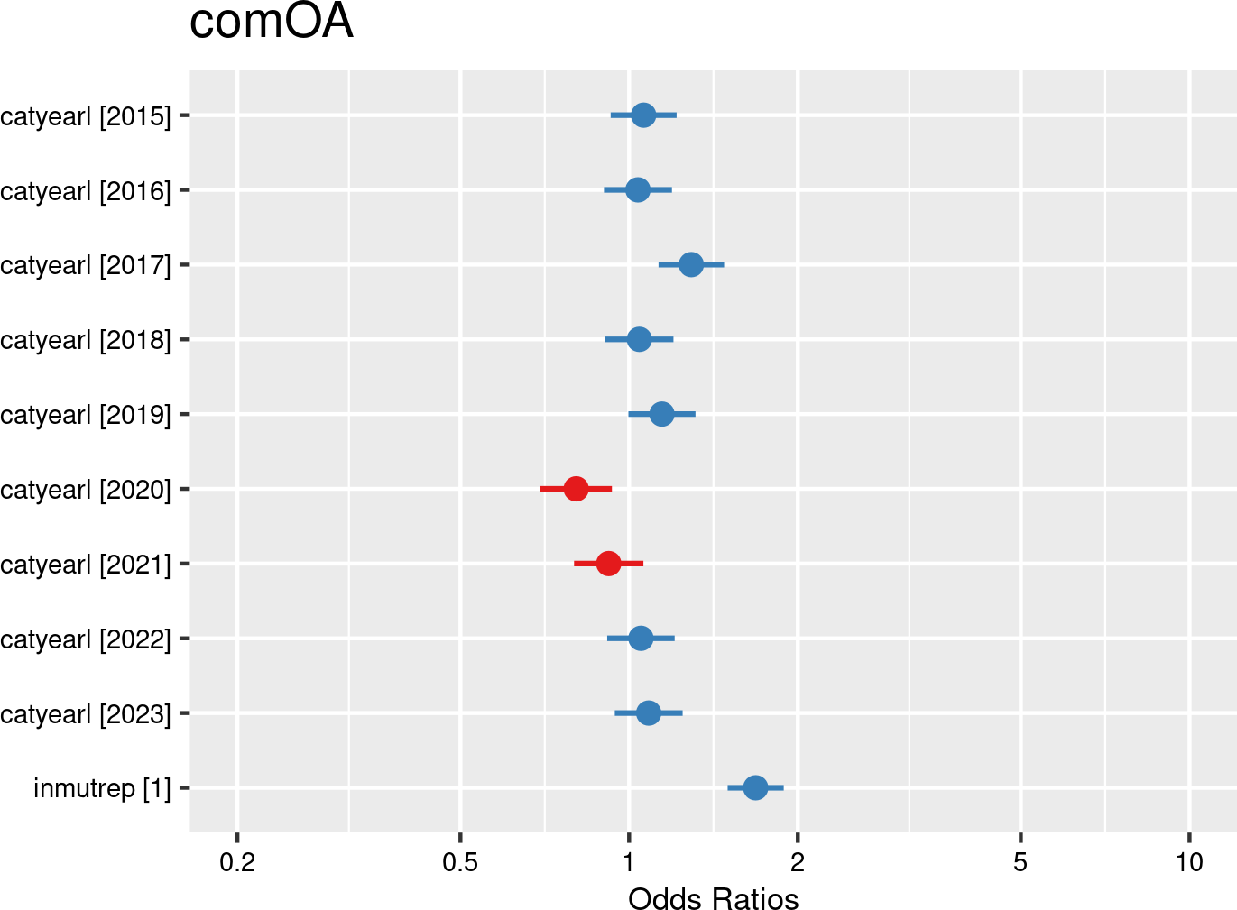

Years were introduced as fixed effects, and companies and employees as random effects. The model is based on data of a sample of 50.000 workers. The model is adjusted for representativeness of the company (fixed effect inmutrep) regarding to sector, size and Flemish province.
Figure 3.198 (a) and Figure 3.198 (b) show that, compared to the reference year 2014, the likelihoods for experiencing workplace occupational accidents were significantly lower in almost all years with exception of 2016; a general decreasing trend in odds ratios is observed over the years.
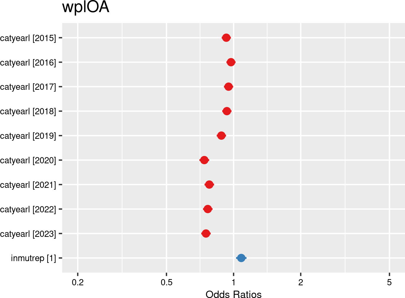

Years were introduced as fixed effects, and companies and employees as random effects. The model is based on data of a sample of 50.000 workers. The model is adjusted for representativeness of the company (fixed effect inmutrep) regarding to sector, size and Flemish province.
Figure 3.199 (a) and Figure 3.199 (b) present a model estimating the frequency degree of OA at the company level. These figures indicate a general and significant decreasing trend in frequency degree estimates over the years compared to the reference year 2014.
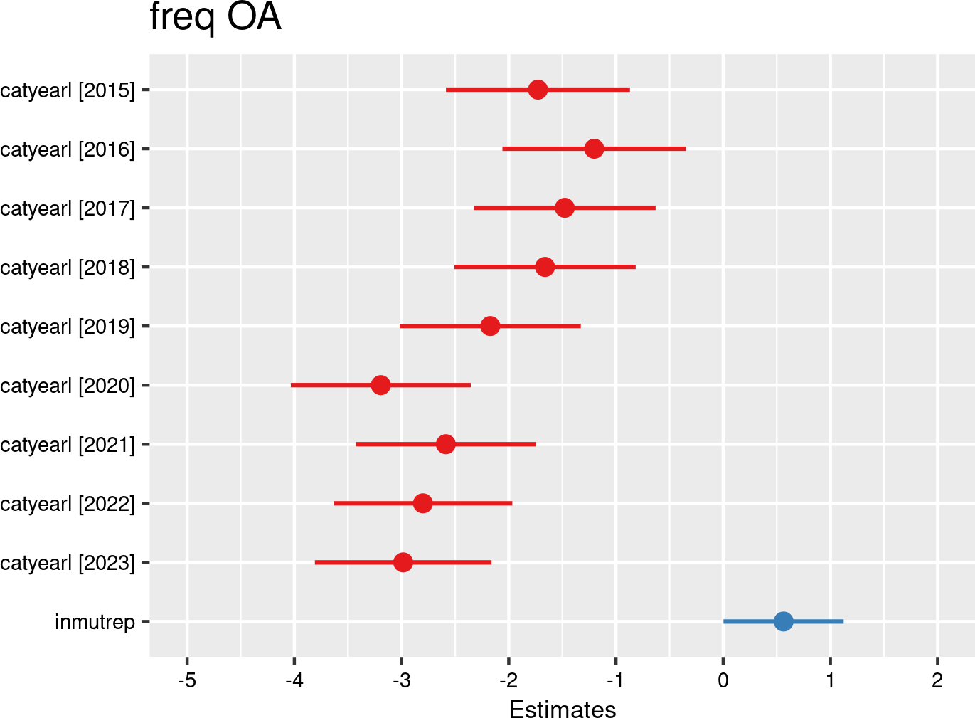

Figure 3.200 (a) and Figure 3.200 (b) present a model estimating the chance for an accepted accident being serious (according to the definition of the Belgian law). These figures indicate that the likelihoods for experiencing serious accidents were significantly higher in 2020 and 2023 compared to the reference year 2014.
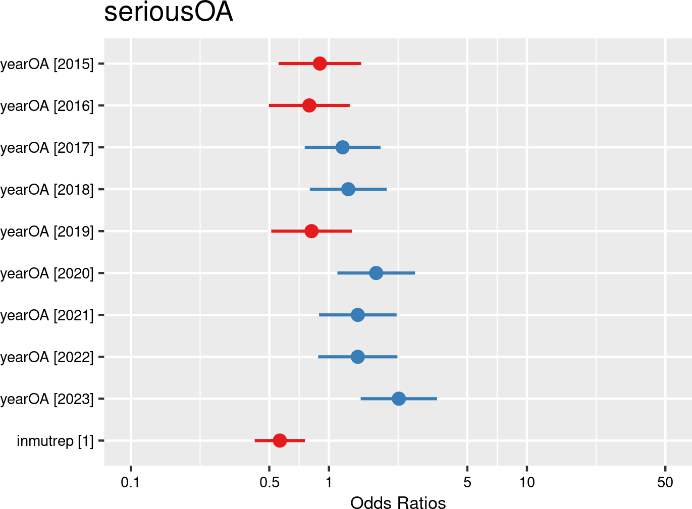

Figure 3.201 (a) and Figure 3.201 (b) show that, compared to the reference year 2014, the numbers of absence days associated with an accepted workplace OA were significantly higher in 2019, 2021 and 2022.
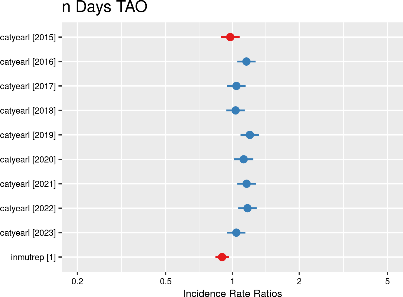

Figure 3.202 (a) and Figure 3.202 (b) confirm the results of the previous model with validated days, showing that the numbers of absence days associated with an accepted workplace OA were significantly higher in 2019, 2021 and 2022.
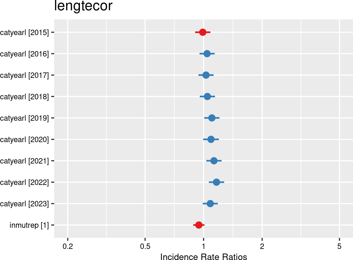

As shown in Figure 3.203 (a) and Figure 3.203 (b), the estimated costs associated with OA were significantly higher in all years compared to the reference year 2014. With the exception of 2018, these costs exhibited a generally increasing trend up to 2021. Although a slight decline is observed in 2022 and 2023, the estimates remain substantially above the 2014 baseline.
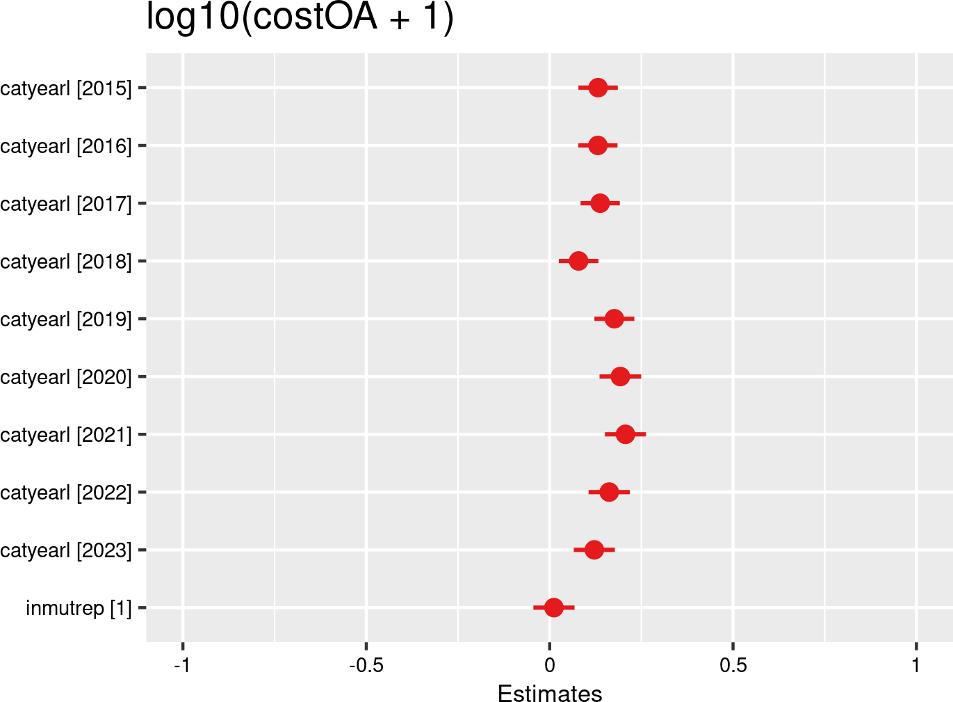

The next 4 figures (Figure 3.204 (a) and Figure 3.204 (b), Figure 3.205 (a) and Figure 3.205 (b)) are displaying the results of models assessing the severity degree of a company in relation to the different years of the study. According to Figure 3.204 (a) and Figure 3.204 (b), only 2023 shows a significantly lower severity degree estimate (based on the validated number of absence days) compared to the reference year 2014.
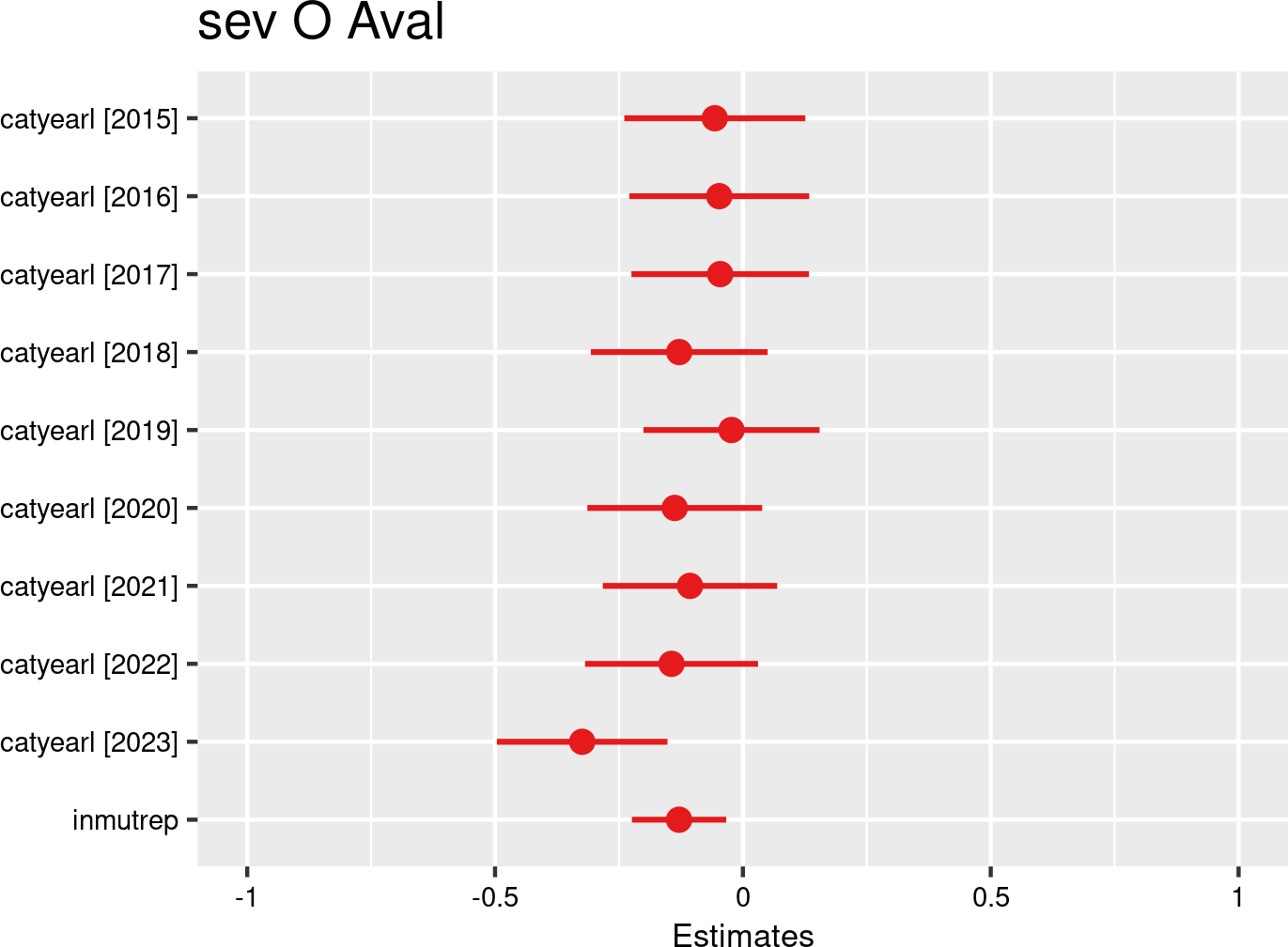

Figure 3.205 (a) and Figure 3.205 (b) (using Liantis PS calculated absence days) partially confirm the results of the previous model with validated days. Here, years 2020 to 2023 exhibit significantly lower severity degree estimates compared to the reference year 2014.
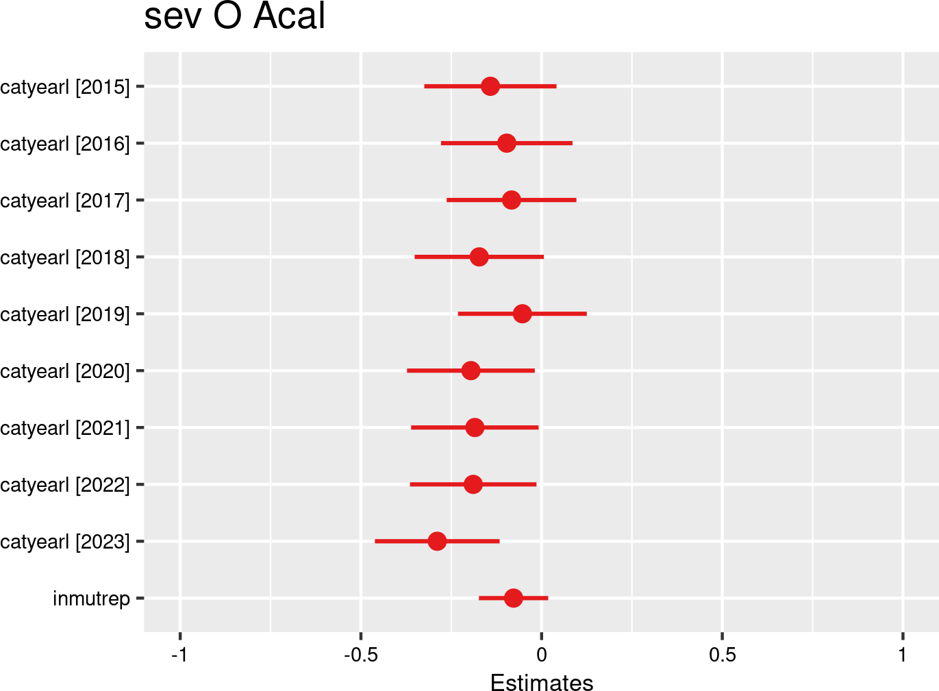

3.4.5.2 Time of the year (months)
3.4.5.2.1 Descriptives
Fedris provides statistics on month of accident. From Liantis PS data it is also possible to derive the month of the wage calculations. The notification contains the date of the OA from which month can be extracted.
all accepted occupational accidents
| monthOAf | rszall | rszpriv | liaall | fedrisall | totalnot | totalnotmut | totalnotrepmutflan |
|---|---|---|---|---|---|---|---|
| January | NA | NA | 1417084 | 124572 | 17642 | 5600 | 2476 |
| February | NA | NA | 1431180 | 114448 | 16359 | 5129 | 2152 |
| March | NA | NA | 1453499 | 119297 | 17104 | 5360 | 2297 |
| April | NA | NA | 1489048 | 100418 | 14670 | 4560 | 1912 |
| May | NA | NA | 1493678 | 106381 | 15315 | 4734 | 2006 |
| June | NA | NA | 1523104 | 122525 | 17756 | 5548 | 2311 |
| July | NA | NA | 1562970 | 97404 | 13948 | 4311 | 1909 |
| August | NA | NA | 1565079 | 107211 | 15530 | 4938 | 2065 |
| September | NA | NA | 1547325 | 122914 | 18259 | 5729 | 2320 |
| October | NA | NA | 1536877 | 124753 | 18391 | 5788 | 2406 |
| November | NA | NA | 1519519 | 112742 | 15996 | 4948 | 2158 |
| December | NA | NA | 1516503 | 100712 | 14249 | 4590 | 2018 |
| monthOAf | percrszall | percrszpriv | percliaall | percfedrisall | perctotalnot | perctotalnotmut | perctotalnotrepmutflan |
|---|---|---|---|---|---|---|---|
| January | NA | NA | 7.85 | 9.20 | 9.04 | 9.15 | 9.51 |
| February | NA | NA | 7.93 | 8.46 | 8.38 | 8.38 | 8.27 |
| March | NA | NA | 8.05 | 8.81 | 8.76 | 8.75 | 8.82 |
| April | NA | NA | 8.25 | 7.42 | 7.51 | 7.45 | 7.35 |
| May | NA | NA | 8.27 | 7.86 | 7.85 | 7.73 | 7.71 |
| June | NA | NA | 8.44 | 9.05 | 9.10 | 9.06 | 8.88 |
| July | NA | NA | 8.66 | 7.20 | 7.14 | 7.04 | 7.33 |
| August | NA | NA | 8.67 | 7.92 | 7.96 | 8.06 | 7.93 |
| September | NA | NA | 8.57 | 9.08 | 9.35 | 9.36 | 8.91 |
| October | NA | NA | 8.51 | 9.22 | 9.42 | 9.45 | 9.24 |
| November | NA | NA | 8.42 | 8.33 | 8.19 | 8.08 | 8.29 |
| December | NA | NA | 8.40 | 7.44 | 7.30 | 7.50 | 7.75 |
commuting accepted occupational accidents
| monthOAf | rszall | rszpriv | liaall | fedrisall | totalnot | totalnotmut | totalnotrepmutflan |
|---|---|---|---|---|---|---|---|
| January | NA | NA | 1417084 | 26825 | 3460 | 1022 | 525 |
| February | NA | NA | 1431180 | 19726 | 2511 | 751 | 366 |
| March | NA | NA | 1453499 | 17935 | 2203 | 679 | 314 |
| April | NA | NA | 1489048 | 14433 | 1789 | 531 | 230 |
| May | NA | NA | 1493678 | 16193 | 2022 | 611 | 303 |
| June | NA | NA | 1523104 | 18887 | 2300 | 686 | 317 |
| July | NA | NA | 1562970 | 14265 | 1615 | 478 | 228 |
| August | NA | NA | 1565079 | 15637 | 2020 | 610 | 291 |
| September | NA | NA | 1547325 | 19919 | 2453 | 754 | 368 |
| October | NA | NA | 1536877 | 21508 | 2754 | 835 | 379 |
| November | NA | NA | 1519519 | 20864 | 2561 | 778 | 379 |
| December | NA | NA | 1516503 | 20118 | 2699 | 864 | 412 |
| monthOAf | percrszall | percrszpriv | percliaall | percfedrisall | perctotalnot | perctotalnotmut | perctotalnotrepmutflan |
|---|---|---|---|---|---|---|---|
| January | NA | NA | 7.85 | 11.85 | 12.19 | 11.89 | 12.77 |
| February | NA | NA | 7.93 | 8.72 | 8.85 | 8.73 | 8.90 |
| March | NA | NA | 8.05 | 7.92 | 7.76 | 7.90 | 7.64 |
| April | NA | NA | 8.25 | 6.38 | 6.30 | 6.18 | 5.59 |
| May | NA | NA | 8.27 | 7.16 | 7.12 | 7.11 | 7.37 |
| June | NA | NA | 8.44 | 8.35 | 8.10 | 7.98 | 7.71 |
| July | NA | NA | 8.66 | 6.30 | 5.69 | 5.56 | 5.54 |
| August | NA | NA | 8.67 | 6.91 | 7.12 | 7.09 | 7.08 |
| September | NA | NA | 8.57 | 8.80 | 8.64 | 8.77 | 8.95 |
| October | NA | NA | 8.51 | 9.50 | 9.70 | 9.71 | 9.22 |
| November | NA | NA | 8.42 | 9.22 | 9.02 | 9.05 | 9.22 |
| December | NA | NA | 8.40 | 8.89 | 9.51 | 10.05 | 10.02 |
workplace accepted occupational accidents
| monthOAf | rszall | rszpriv | liaall | fedrisall | totalnot | totalnotmut | totalnotrepmutflan |
|---|---|---|---|---|---|---|---|
| January | NA | NA | 1417084 | 97747 | 14182 | 4578 | 1951 |
| February | NA | NA | 1431180 | 94722 | 13848 | 4378 | 1786 |
| March | NA | NA | 1453499 | 101362 | 14901 | 4681 | 1983 |
| April | NA | NA | 1489048 | 85985 | 12881 | 4029 | 1682 |
| May | NA | NA | 1493678 | 90188 | 13293 | 4123 | 1703 |
| June | NA | NA | 1523104 | 103638 | 15456 | 4862 | 1994 |
| July | NA | NA | 1562970 | 83139 | 12333 | 3833 | 1681 |
| August | NA | NA | 1565079 | 91574 | 13510 | 4328 | 1774 |
| September | NA | NA | 1547325 | 102995 | 15806 | 4975 | 1952 |
| October | NA | NA | 1536877 | 103245 | 15637 | 4953 | 2027 |
| November | NA | NA | 1519519 | 91878 | 13435 | 4170 | 1779 |
| December | NA | NA | 1516503 | 80594 | 11550 | 3726 | 1606 |
| monthOAf | percrszall | percrszpriv | percliaall | percfedrisall | perctotalnot | perctotalnotmut | perctotalnotrepmutflan |
|---|---|---|---|---|---|---|---|
| January | NA | NA | 7.85 | 8.67 | 8.50 | 8.70 | 8.90 |
| February | NA | NA | 7.93 | 8.40 | 8.30 | 8.32 | 8.15 |
| March | NA | NA | 8.05 | 8.99 | 8.93 | 8.89 | 9.05 |
| April | NA | NA | 8.25 | 7.63 | 7.72 | 7.65 | 7.67 |
| May | NA | NA | 8.27 | 8.00 | 7.97 | 7.83 | 7.77 |
| June | NA | NA | 8.44 | 9.20 | 9.26 | 9.24 | 9.10 |
| July | NA | NA | 8.66 | 7.38 | 7.39 | 7.28 | 7.67 |
| August | NA | NA | 8.67 | 8.12 | 8.10 | 8.22 | 8.09 |
| September | NA | NA | 8.57 | 9.14 | 9.47 | 9.45 | 8.91 |
| October | NA | NA | 8.51 | 9.16 | 9.37 | 9.41 | 9.25 |
| November | NA | NA | 8.42 | 8.15 | 8.05 | 7.92 | 8.12 |
| December | NA | NA | 8.40 | 7.15 | 6.92 | 7.08 | 7.33 |
3.4.5.2.2 Models
The following Table 3.136 table summarizes the results of the models assessing the relationship between the different years of the study and the several outcomes related to OAs. Below the table, details are provided about the data used for the analyses. The results of the nine models are then presented both graphically and in a table.
| catmonth | chance to notify | chance on refusal | chance commuting | chance workplace | freq degree | chance serious | nDays TAO V/C | cost | sev degree V/C |
|---|---|---|---|---|---|---|---|---|---|
| Jan | REF | REF | REF | REF | ns | REF | REF | REF | REF |
| Feb | ns | ns | ns | ns | > | ns | ns | ns | ns |
| Mar | < | ns | < | ns | > | < | ns | < | > |
| Apr | < | ns | < | < | > | ns | ns/< | ns | > |
| May | < | ns | < | < | > | ns | </ns | < | ns |
| Jun | ns | ns | < | ns | > | ns | ns/< | ns | ns |
| Jul | < | ns | < | < | > | ns | </< | < | ns |
| Aug | < | ns | < | < | > | ns | </< | < | ns |
| Sep | ns | ns | < | ns | > | ns | ns | ns | ns |
| Oct | ns | ns | < | > | > | ns | ns | < | > |
| Nov | ns | ns | < | ns | > | ns | ns | ns | ns |
| Dec | < | ns | < | < | rank def | ns | ns | < | rank def |
| occur | accept | occur | occur | occur | severe | severe | severe | severe | |
| empl | empl | empl | empl | comp | empl | empl | empl | comp | |
| c/w all | c/w ref | c acc | w acc | w acc | w acc | w acc | w acc | w acc |
- occur: data include all workers, chance for occurrence is calculated for the outcome
- accept: data include only workers with a notification of OA
- severe: data include only workers with an accepted OA
- c/w all: commuting and workplace accidents, including refused and accidents without decisions
- c/w ref: accepted or refused commuting and workplace accidents
- c acc: accepted commuting accidents
- w acc: accepted workplace accidents
- empl: the outcome is situated at the individual level
- comp: the outcome is situated at the company level
- nDaysTAO: number of days absenteeism related to the OA
- V/C: Validated number of days (available from FEDRIS) / Calculated number of days (based on the Liantis PS data)
Time of the year (months) and occupational accidents
- Compared to reference month January, the likelihoods to notify were significantly lower in March, April, May, July, August and December
- No significant differences were observed for the likelihoods for refusal across months
- The likelihoods for experiencing commuting occupational accidents were significantly lower in all months but February
- For workplace occupational accidents, the likelihoods were significantly lower in April, May, July, August and December; highest estimates were observed September, February, June and October, but only for October the increase was significant in comparison with January
- The likelihoods for experiencing serious accidents were significantly lower in March compared to January
- Absence days (validated and calculated) were lower in July and August
- Costs related to occupational accidents were significantly lower in March, May, July, August, October and December; these are also the months with 31 days and smaller confidence intervals
From Figure 3.206 (a) and Figure 3.206 (b) we learn that, compared to the reference month January, the likelihoods to notify were significantly lower in March, April, May, July, August and December.
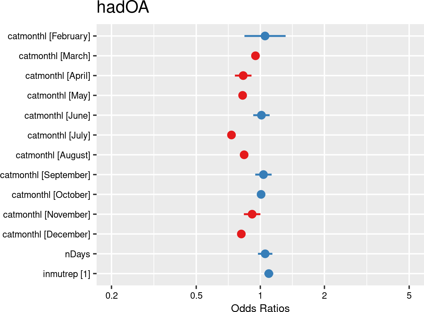

Months were introduced as fixed effects, and companies and employees as random effects. The model is based on data of a sample of 50,000 workers. The model is adjusted for representativeness of the company (fixed effect inmutrep) regarding to sector, size and Flemish province.
According to Figure 3.207 (a) and Figure 3.207 (b), no significant differences were observed for the likelihoods for refusal across months compared to the reference month January.
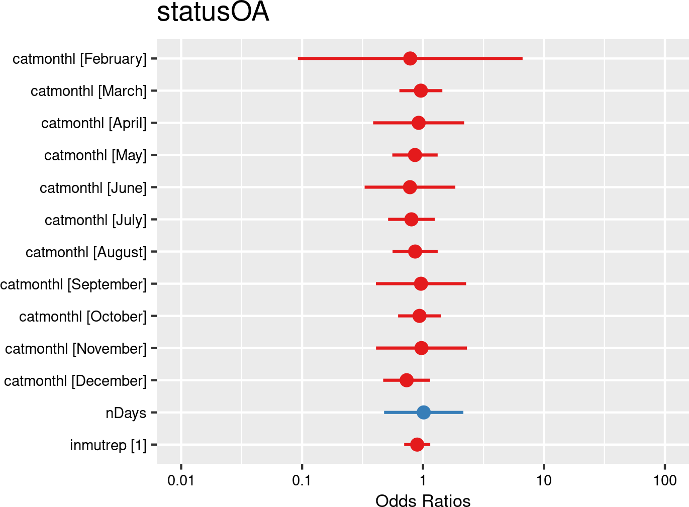

Months were introduced as fixed effects, and companies and employees as random effects. The model is based on data of all employees. The model is adjusted for representativeness of the company (fixed effect inmutrep) regarding to sector, size and Flemish province.
According to Figure 3.208 (a) and Figure 3.208 (b), the likelihoods for experiencing commuting occupational accidents were significantly lower in all months but February compared to the reference month January.
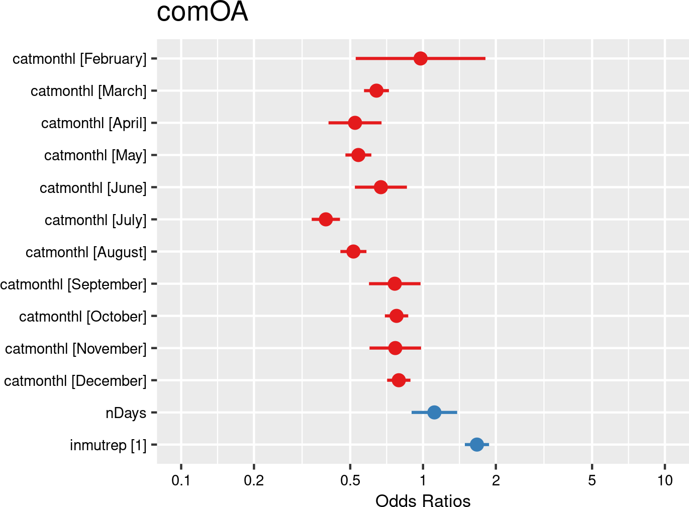

Months were introduced as fixed effects, and companies and employees as random effects. The model is based on data of a sample of 50.000 workers. The model is adjusted for representativeness of the company (fixed effect inmutrep) regarding to sector, size and Flemish province.
Figure 3.209 (a) and Figure 3.209 (b) show that, compared to the reference month January, the likelihoods for experiencing workplace occupational accidents were significantly lower in April, May, July, August and December; highest estimates were observed September, February, June and October, but only for October the increase was significant in comparison with January.
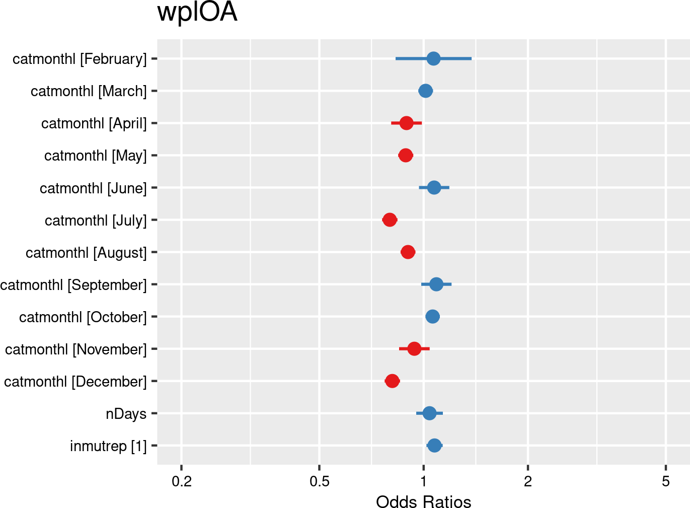

Months were introduced as fixed effects, and companies and employees as random effects. The model is based on data of a sample of 50.000 workers. The model is adjusted for representativeness of the company (fixed effect inmutrep) regarding to sector, size and Flemish province.
Figure 3.210 (a) and Figure 3.210 (b) present a model estimating the frequency degree of OA at the company level. These figures indicate that the frequency degree estimates are significantly influenced by fractions of employees at work in all months but January and December.
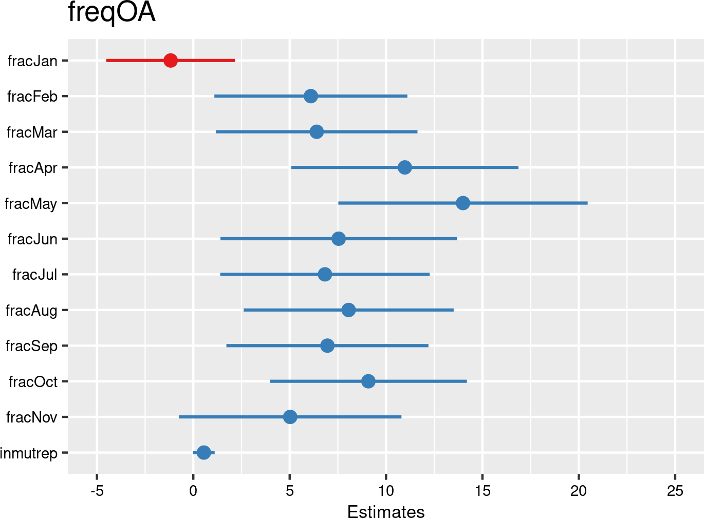

Figure 3.211 (a) and Figure 3.211 (b) present a model estimating the chance for an accepted workplace OA being serious (according to the definition of the Belgian law). These figures indicate that the likelihoods for experiencing serious accidents were significantly lower in March compared to January.
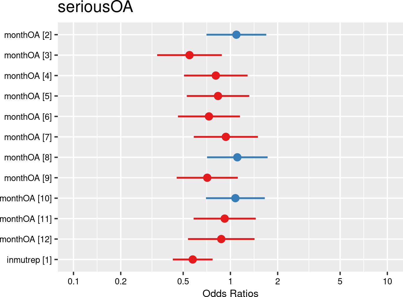

Figure 3.212 (a) and Figure 3.212 (b) show that, compared to the reference month January, absence days (validated and calculated) were lower in July and August.
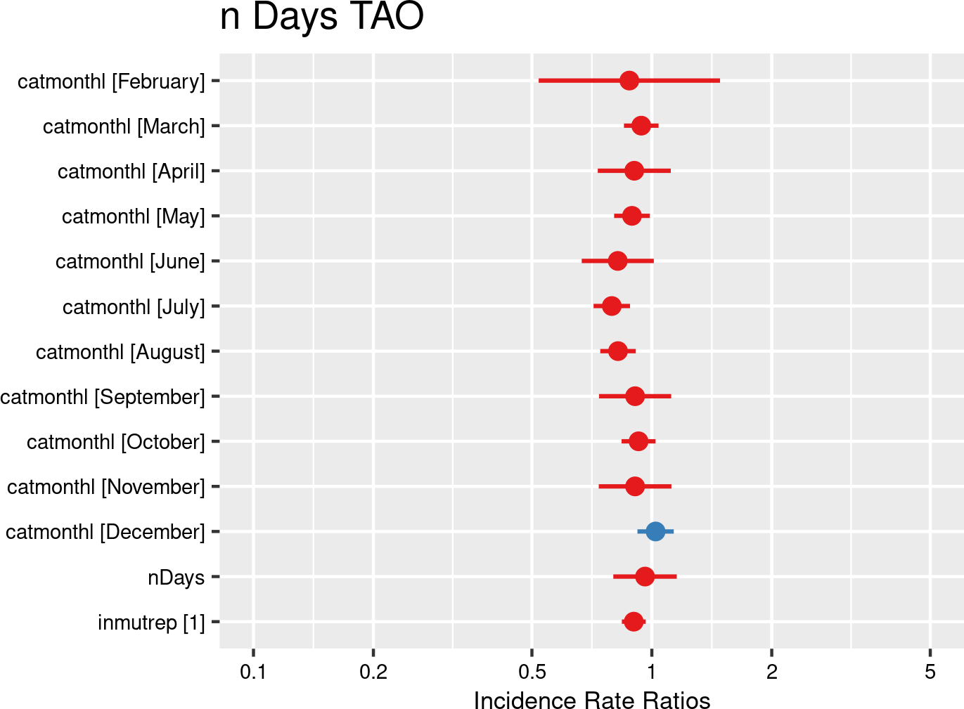

Figure 3.213 (a) and Figure 3.213 (b) largely confirm the results of the previous model with validated days.
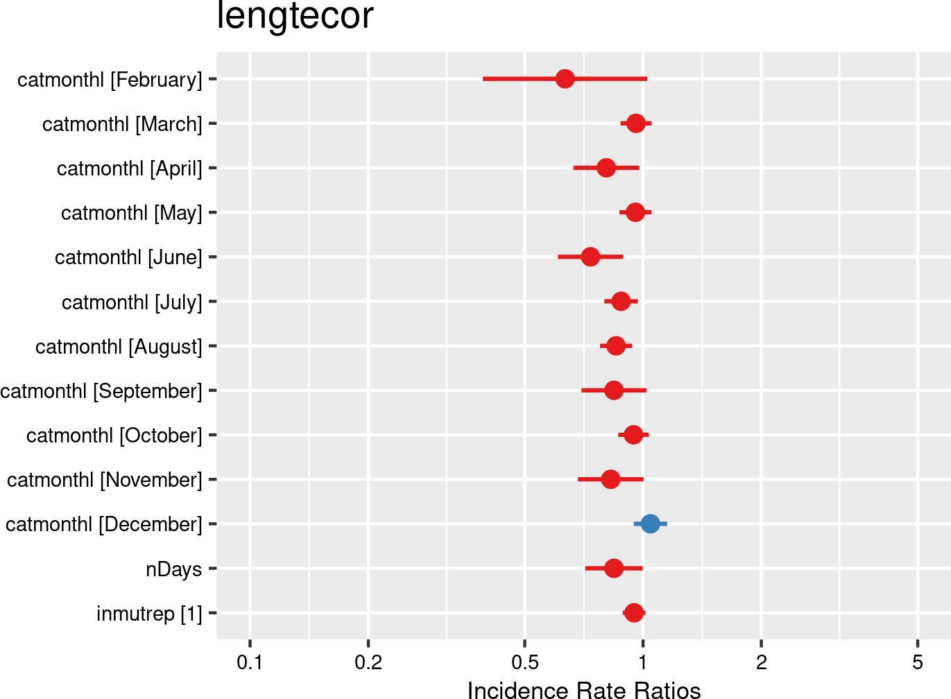

Figure 3.214 (a) and Figure 3.214 (b) show that, compared to the reference month January, costs related to occupational accidents were significantly lower in March, May, July, August, October and December; these are also the months with 31 days and smaller confidence intervals on the estimates.
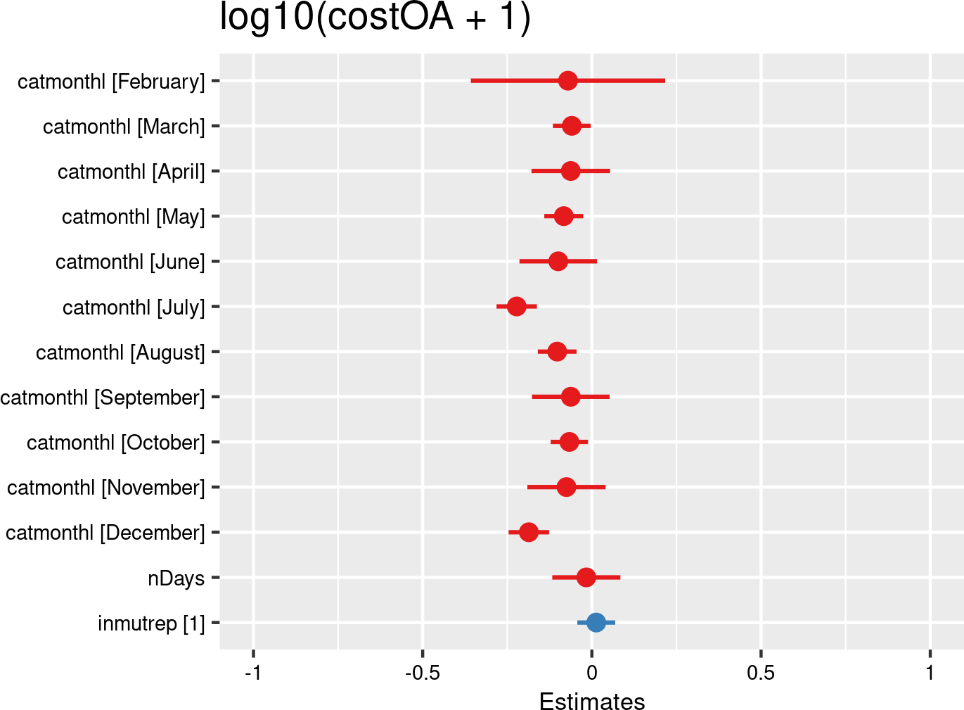

The next 4 figures (Figure 3.215 (a) and Figure 3.215 (b), Figure 3.216 (a) and Figure 3.216 (b)) are displaying the results of models assessing the severity degree of a company using employment fractions accross the different months of the year. According to Figure 3.215 (a) and Figure 3.215 (b), employment fractions from March, April and October seem to have a larger impact.
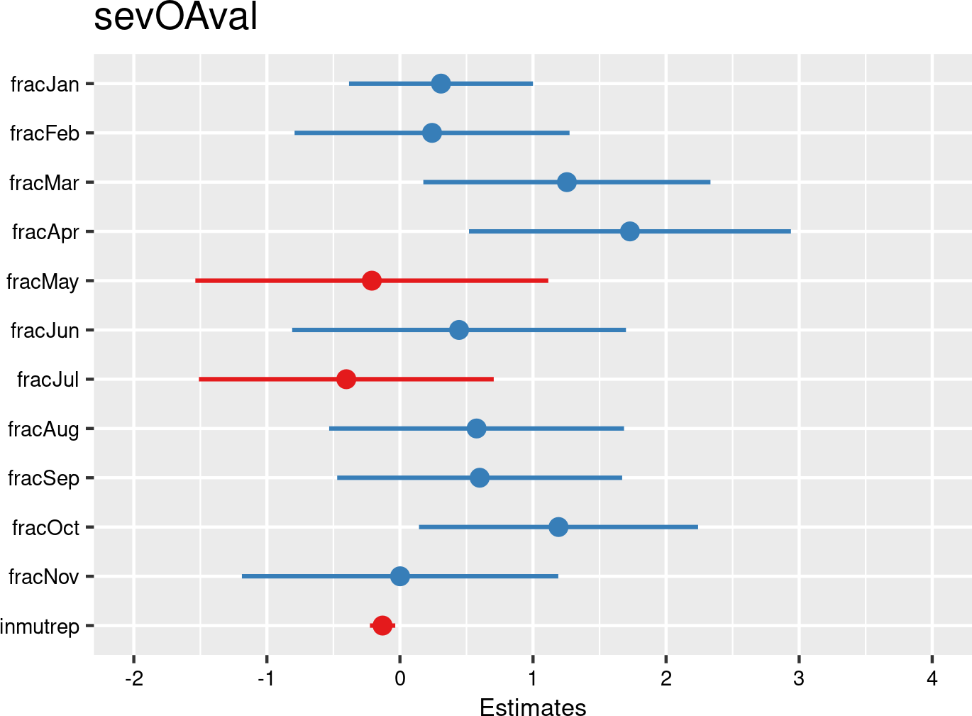

Figure 3.216 (a) and Figure 3.216 (b) (using Liantis PS calculated absence days) show an image analogous to the previous model with validated days, although no significant results are found here.
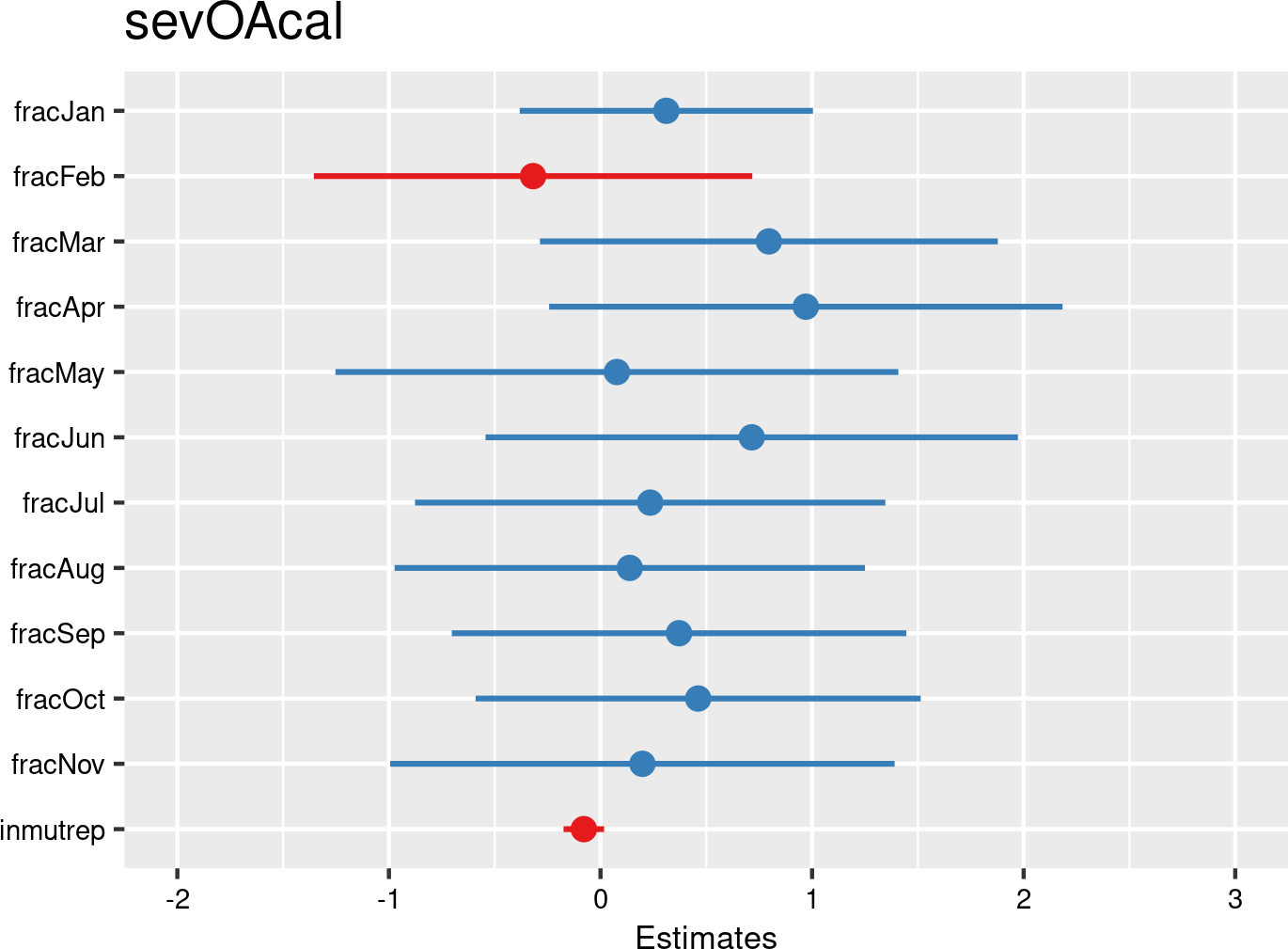

3.4.5.3 Time of the week (days)
Data Quality Alert: time of the week (days)
- Although Liantis holds detailed data on the number of people actually at work on each individual day across the ten-year study period, this level of granularity was not accessible within the scope of the present project.
- For previous models, monthly-level data on wages and worked hours provided sufficient detail. However, to construct a model assessing the likelihood of experiencing an occupational accident on a specific weekday, this granularity is insufficient.
- As a result, it was not possible to build weekday-level models comparable to earlier analyses. Specifically, no models can be constructed to investigate the impact of the day of the week on the likelihood to notify (or experience) an occupational (commuting or workplace) accident.
- Instead, for the current and subsequent models exploring temporal and calendar effects, we opted to use all available Liantis ESPP OA notification data or for commuting or for workplace accidents.
- This represents a fundamentally different approach, and it is important to remain aware of this methodological shift in this part of the report.
The number of OA notifications by weekday for commuting and workplace accidents is summarized in Table 3.137.
| wdayOA | n_comOA | n_wplOA | perc_comOA_c | perc_wplOA_c | perc_comOA_r | perc_wplOA_r |
|---|---|---|---|---|---|---|
| Monday | 6574 | 37402 | 20.2 | 20.3 | 14.9 | 85.1 |
| Tuesday | 6685 | 36713 | 20.6 | 19.9 | 15.4 | 84.6 |
| Wednesday | 5936 | 34610 | 18.3 | 18.8 | 14.6 | 85.4 |
| Thursday | 6174 | 33566 | 19.0 | 18.2 | 15.5 | 84.5 |
| Friday | 5203 | 28141 | 16.0 | 15.3 | 15.6 | 84.4 |
| Saturday | 1151 | 7974 | 3.5 | 4.3 | 12.6 | 87.4 |
| Sunday | 801 | 6016 | 2.5 | 3.3 | 11.8 | 88.2 |
In absolute terms, both commuting and workplace OA notifications peak on Mondays and are least frequent on Saturdays and Sundays. The weekday distribution of OA notifications differs significantly between commuting and workplace accidents (\(\chi^2 = 125.53\), \(df = 6\), \(p < 0.001\)). This pattern aligns with previous findings from Medex on OA in the public sector (Federal Public Service Health, Food Chain Safety and Environment, 2022). Notably, the proportion of workplace OA increases during weekends compared to weekdays, a trend also observed in the Medex study. However, the relative shares differ: approximately 15% commuting and 85% workplace in the present study (2014–2023) versus 25% and 75% in Medex (2016–2020). The lower number of OA on Wednesdays reported by Medex -attributed to higher telework and/or part-time work- was not confirmed in our study. Overall, our findings align with the broader literature discussed in Section 1.3.6.3.
Time of the week (days) and occupational accidents
- Most occupational accidents -both commuting and workplace- occur on Mondays and Tuesdays.
- The fewest occupational accidents (commuting and workplace) occur on Saturdays and Sundays.
- However, the proportion of workplace accidents increases during weekends compared to weekdays.
3.4.5.4 Time of the day (hours)
Data Quality Alert: time of the day (hours)
- Although Liantis holds detailed data on the number of people actually at work on each individual day across the ten-year study period, this level of granularity was not accessible within the scope of the present project.
- As a result, it was not possible to build within-day-level models. Specifically, no models can be constructed to investigate the impact of the hour of the day on the likelihood to notify (or experience) an occupational (commuting or workplace) accident.
- Instead, for the current and subsequent models exploring temporal and calendar effects, we opted to use all available Liantis ESPP OA notification data or for commuting or for workplace accidents.
- This represents a fundamentally different approach, and it is important to remain aware of this methodological shift in this part of the report.
The number of OA notifications by hour of the day for commuting and workplace accidents is summarized in Table 3.138.
| hourOA | n_comOA | n_wplOA | perc_comOA_c | perc_wplOA_c | perc_comOA_r | perc_wplOA_r |
|---|---|---|---|---|---|---|
| 00:00:00 | 176 | 1872 | 0.6 | 1.0 | 8.6 | 91.4 |
| 01:00:00 | 53 | 1093 | 0.2 | 0.6 | 4.6 | 95.4 |
| 02:00:00 | 43 | 929 | 0.1 | 0.5 | 4.4 | 95.6 |
| 03:00:00 | 68 | 988 | 0.2 | 0.6 | 6.4 | 93.6 |
| 04:00:00 | 413 | 1155 | 1.3 | 0.6 | 26.3 | 73.7 |
| 05:00:00 | 1143 | 1646 | 3.6 | 0.9 | 41.0 | 59.0 |
| 06:00:00 | 2861 | 3422 | 9.0 | 1.9 | 45.5 | 54.5 |
| 07:00:00 | 6346 | 7529 | 20.0 | 4.2 | 45.7 | 54.3 |
| 08:00:00 | 4371 | 14167 | 13.8 | 7.9 | 23.6 | 76.4 |
| 09:00:00 | 970 | 16725 | 3.1 | 9.4 | 5.5 | 94.5 |
| 10:00:00 | 508 | 22054 | 1.6 | 12.4 | 2.3 | 97.7 |
| 11:00:00 | 617 | 20515 | 1.9 | 11.5 | 2.9 | 97.1 |
| 12:00:00 | 1796 | 9765 | 5.7 | 5.5 | 15.5 | 84.5 |
| 13:00:00 | 1422 | 12897 | 4.5 | 7.2 | 9.9 | 90.1 |
| 14:00:00 | 905 | 16406 | 2.8 | 9.2 | 5.2 | 94.8 |
| 15:00:00 | 1205 | 15729 | 3.8 | 8.8 | 7.1 | 92.9 |
| 16:00:00 | 2677 | 10263 | 8.4 | 5.8 | 20.7 | 79.3 |
| 17:00:00 | 2918 | 5359 | 9.2 | 3.0 | 35.3 | 64.7 |
| 18:00:00 | 1332 | 4172 | 4.2 | 2.3 | 24.2 | 75.8 |
| 19:00:00 | 443 | 3297 | 1.4 | 1.8 | 11.8 | 88.2 |
| 20:00:00 | 428 | 3036 | 1.3 | 1.7 | 12.4 | 87.6 |
| 21:00:00 | 515 | 2347 | 1.6 | 1.3 | 18.0 | 82.0 |
| 22:00:00 | 428 | 1636 | 1.3 | 0.9 | 20.7 | 79.3 |
| 23:00:00 | 122 | 1467 | 0.4 | 0.8 | 7.7 | 92.3 |
| NA | 764 | 5953 | NA | NA | 11.4 | 88.6 |
The result is also graphically presented in Figure 3.217.
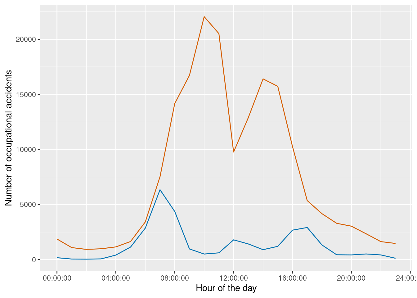
Commuting accidents peak in the early morning (before 08:00) and evening (after 17:00), with a smaller peak around noon. Workplace accidents increase sharply from 06:00, reaching peaks at 10:00–11:00 and 14:00–15:00, and decline around noon and after 16:00. Between 05:00–08:00, at 12:00, and after 16:00, the proportion of commuting OA rises relative to workplace OA (see Table 3.138), reflecting typical home-to-work and return travel times. This pattern is consistent with the literature overview in Section 1.3.6.4. The difference in hourly distribution between commuting and workplace accidents is statistically significant (\(\chi^2 = 30483\), \(df = 24\), \(p < 0.001\)).
Time of the day (hours) and occupational accidents
- Commuting accidents peak in the early morning (before 08:00) and evening (after 17:00), with a smaller peak around noon.
- Workplace accidents increase sharply from 06:00, reaching peaks at 10:00–11:00 and 14:00–15:00, and decline around noon and after 16:00.
- The proportion of commuting accidents rises relative to workplace accidents during typical home-to-work and return travel times (05:00–08:00, 12:00, and after 16:00).
3.4.5.5 Weather
In Section 2.18.3 is described how weather data were collected. Table 2.106 showed that more extreme weather conditions such as freezing temperatures and heatwaves are relatively uncommon (1.94% of days and 2.67% of days respectively in the source dataset).
We take those two conditions as an example to illustrate whether, when these conditions do occur, they influence the distribution of commuting versus workplace accidents.
The number of OA notifications by freezing conditions (maximum temperatures below zero) for commuting and workplace accidents is summarized in Table 3.139.
| temp_freezing | n_comOA | n_wplOA | perc_comOA_c | perc_wplOA_c | perc_comOA_r | perc_wplOA_r |
|---|---|---|---|---|---|---|
| 0 | 30923 | 164196 | 97.2 | 98.2 | 15.8 | 84.2 |
| 1 | 899 | 3022 | 2.8 | 1.8 | 22.9 | 77.1 |
| NA | 421 | 14948 | NA | NA | 2.7 | 97.3 |
The number of OA notifications by heatwave conditions (maximum temperatures in Uccle \(\geq\) 25°C for at least five consecutive days, with at least three \(\geq\) 30°C) for commuting and workplace OA is summarized in Table 3.140.
| heatwave | n_comOA | n_wplOA | perc_comOA_c | perc_wplOA_c | perc_comOA_r | perc_wplOA_r |
|---|---|---|---|---|---|---|
| 0 | 31007 | 162595 | 97.4 | 97.2 | 16.0 | 84.0 |
| 1 | 815 | 4623 | 2.6 | 2.8 | 15.0 | 85.0 |
| NA | 421 | 14948 | NA | NA | 2.7 | 97.3 |
Freezing conditions are associated with a higher proportion of commuting OA (22.9%) compared to non-freezing conditions (15.8%) (see Table 3.139), a difference that is statistically significant (\(\chi^2 = 142.9\), \(df = 1\), \(p < 0.001\)). Heatwave conditions also show a significant difference in the proportion of commuting OA (15.0%) compared to non-heatwave conditions (16.0%) (see Table 3.140) (\(\chi^2 = 4.1\), \(df = 1\), \(p = 0.043\)). These findings suggest that freezing weather may increase the risk of commuting OA, whereas heatwaves may shift risk toward more workplace OA. Both observations are consistent with previous research discussed in Section 1.3.6.5. Further research should examine the mechanisms underlying these patterns and assess whether they persist after adjusting for other variables. Such a model is presented in Section 3.4.5.10.
Weather and occupational accidents
- Extreme weather conditions appear to influence the distribution of commuting and workplace accidents.
- Heatwaves are associated with a relative increase in workplace accidents, whereas freezing conditions are linked to a relative increase in commuting accidents.
3.4.5.6 Holidays & vacations
In Section 2.18.1 is described how the calendar with Belgian holidays was constructed (see Table 2.100, Table 2.101 and Table 2.102).
We take the Belgian school holidays (Herfstvakantie, Kerstvakantie, Krokusvakantie, Paasvakantie, Zomervakantie) and legal holidays (Allerheiligen, Dag van de arbeid, Kerstmis, Nationale feestdag van België, Nieuwjaar, Onze-Lieve-Heer-Hemelvaart, Onze-Lieve-Vrouw-Hemelvaart/Moederdag Antwerpen, Paasmaandag, Pasen, Pinksteren, Pinkstermaandag, Wapenstilstand/Sint-Maarten) as examples to illustrate whether, when these conditions do occur, they influence the distribution of commuting versus workplace accidents.
The distribution of commuting and workplace OA across school holiday periods is summarized in Table 3.141.
| schoolhol | n_comOA | n_wplOA | perc_comOA_c | perc_wplOA_c | perc_comOA_r | perc_wplOA_r |
|---|---|---|---|---|---|---|
| 0 | 25596 | 139865 | 78.7 | 75.8 | 15.5 | 84.5 |
| 1 | 6928 | 44557 | 21.3 | 24.2 | 13.5 | 86.5 |
The distribution of commuting and workplace OA across legal holidays and non-holidays is summarized in Table 3.142.
| legalhol | n_comOA | n_wplOA | perc_comOA_c | perc_wplOA_c | perc_comOA_r | perc_wplOA_r |
|---|---|---|---|---|---|---|
| 0 | 32354 | 183083 | 99.5 | 99.3 | 15.0 | 85.0 |
| 1 | 170 | 1339 | 0.5 | 0.7 | 11.3 | 88.7 |
Both school holidays and legal holidays are associated with a lower proportion of commuting OA compared to non-holiday periods (see Table 3.141 and Table 3.142), with differences that are statistically significant (school holidays: \(\chi^2 = 124.7\), \(df = 1\), \(p < 0.001\); legal holidays: \(\chi^2 = 16.3\), \(df = 1\), \(p < 0.001\)). The absolute number of accidents is much lower on legal holidays, as most of the Belgian workforce does not work on these days, whereas during school holidays, variation occurs depending on which workers take leave. These findings suggest that both school and legal holidays reduce the risk of commuting OA, likely due to decreased travel during these periods. This is consistent with previous research discussed in Section 1.3.6.6. Further research should examine the mechanisms underlying these patterns and assess whether they persist after adjusting for other variables.
Holidays & vacations and occupational accidents
- Holidays, including school and legal holidays, influence the distribution of commuting and workplace accidents.
- School holidays occur more frequently and are associated with a relative decrease in commuting accidents from 15.5% to 13.5%.
- Legal holidays occur less frequently and are associated with a relative decrease in commuting accidents from 15.0% to 11.3%.
3.4.5.7 Summer- and wintertime changes
In Section 2.18.1 is described how summer- and wintertime changes were included in the calendar (see Table 2.103).
In the present paragraph we analyse whether, when these conditions do occur, they influence the distribution of commuting versus workplace accidents.
The distribution of commuting and workplace OA across timeregimes is summarized in Table 3.143. Chi-square tests were conducted for the second and third rows and the fifth and sixth rows to assess differences in commuting versus workplace accidents in the week before before and after time changes. The relative increase in commuting accidents from 12.3% to 12.5% (week before and after the switch to summertime) and the decrease from 15.0% to 13.5% (week before and after the switch to wintertime) were not statistically significant (\(\chi^2 = 0.05\), \(df = 1\), \(p = 0.819\); \(\chi^2 = 3.27\), \(df = 1\), \(p = 0.071\), respectively). It should be noted however that time changes affect only one hour on two weekend days per year and often coincide with school holidays, limiting statistical power and introducing potential confounding.
| timechangeregime | n_comOA | n_wplOA | perc_comOA_c | perc_wplOA_c | perc_comOA_r | perc_wplOA_r |
|---|---|---|---|---|---|---|
| winter (normal) | 14304 | 68213 | 44.0 | 37.0 | 17.3 | 82.7 |
| end winter (normal) | 516 | 3667 | 1.6 | 2.0 | 12.3 | 87.7 |
| begin summer (less sleep) | 477 | 3330 | 1.5 | 1.8 | 12.5 | 87.5 |
| summer (normal) | 16061 | 102302 | 49.4 | 55.5 | 13.6 | 86.4 |
| end summer (normal) | 740 | 4189 | 2.3 | 2.3 | 15.0 | 85.0 |
| begin winter (more sleep) | 426 | 2721 | 1.3 | 1.5 | 13.5 | 86.5 |
Summer- and wintertime changes and occupational accidents
- Based on the data collected in this study, no significant effect of summer- or wintertime changes on the occurrence of commuting or workplace accidents was detected.
- This does not imply the absence of an effect; rather, any effect is likely small and difficult to detect given the limited observation window (one week before and after two specific dates per year) and the potential confounding influence of school holidays.
3.4.5.8 COVID-19 pandemic
In Section 2.18.2 is described how the COVID-19 measures taken in Belgium were included in the calendar using the COVID-19 stringency index (Hale et al., 2021). See Figure 2.61 for an illustration of the effect.
We arbitrarily categorised the stringency index between 2020-01-01 and 2022-12-31 (3 years) into values above and below 50 to assess its effect on the occurrence of commuting versus workplace accidents and called the period before 2020 (6 years) and after 2023 (1 year) pre and post COVID-19 respectively.
The distribution of commuting and workplace OA across COVID-19 measures, categorized by stringency index, is summarized in Table 3.144. A chi-square test confirmed that the observed differences in commuting versus workplace accidents across categories are statistically significant (\(\chi^2 = 234.01\), \(df = 3\), \(p < 0.001\)). Although not shown in the table, cases before and after COVID-19 account for roughly 60% and 10% of the total (over seven years) for both commuting and workplace OA. Within the remaining 30% of cases (three years), the effect of high versus low stringency index is clear and aligns with expectations.
| covid_stringency | n_comOA | n_wplOA | perc_comOA_c | perc_wplOA_c | perc_comOA_r | perc_wplOA_r |
|---|---|---|---|---|---|---|
| pre COVID-19 | 18844 | 112583 | 57.9 | 61.0 | 14.3 | 85.7 |
| high stringency | 3716 | 22795 | 11.4 | 12.4 | 14.0 | 86.0 |
| low stringency | 6182 | 30928 | 19.0 | 16.8 | 16.7 | 83.3 |
| post COVID-19 | 3782 | 18116 | 11.6 | 9.8 | 17.3 | 82.7 |
COVID-19 pandemic and occupational accidents
- The COVID-19 pandemic and related public health measures significantly affected the distribution of commuting and workplace accidents.
- Periods of high stringency were associated with a marked decrease in commuting accidents (from 16.7% to 14.0%) and a corresponding increase in the proportion of workplace accidents (from 83.3% to 86.0%).
- In absolute terms, higher stringency index values (\(\geq\) 50 was chosen here) coincided with lower overall numbers of OA, for both commuting and workplace accidents.
3.4.5.9 Terrorist attacks
On 22 March 2016, terrorist attacks occurred in Belgium at Brussels Airport and Maelbeek metro station, followed by another attack in Liège on 29 May 2018. A previous report by Medex noted potential effects of these events on OA in the public sector on those days (Federal Public Service Health, Food Chain Safety and Environment, 2022).
Although the list of terrorist attacks in Belgium during the study period is longer, those to attacks to examine whether such events influence the distribution of commuting versus workplace accidents.
The distribution of commuting and workplace OA incidents on days when terrorist attacks occurred is summarized in Table 3.145. Chi-square tests were not conducted due to the exceptional nature of these events and the already established influence of factors such as weekday (see Section 3.4.5.3). For instance, attacks occurring during weekends are expected to coincide with a lower proportion of commuting accidents.
Notably, 22 March 2016 was a Tuesday, a day on which approximately 15.4% of commuting accidents would typically be expected (see Table 3.137). However, following the terrorist attacks at Brussels Airport and Maelbeek metro station, the airport departure hall was evacuated and metro services were suspended. The crisis center advised the public to avoid Brussels and remain at home. Schools, government offices, and many businesses sent staff home, and public transport was largely halted. The observed lower percentage of commuting accidents on that day aligns with these extraordinary circumstances.
| attack | dateTA | wdayTA | n_comOA | n_wplOA | perc_comOA_c | perc_wplOA_c | perc_comOA_r | perc_wplOA_r |
|---|---|---|---|---|---|---|---|---|
| attack 01 | 2014-05-24 | Saturday | 1 | 12 | 0.0 | 0.0 | 7.7 | 92.3 |
| attack 02 | 2014-12-14 | Sunday | 1 | 8 | 0.0 | 0.0 | 11.1 | 88.9 |
| attack 03 | 2015-01-15 | Thursday | 8 | 60 | 0.0 | 0.0 | 11.8 | 88.2 |
| attack 04 | 2016-03-15 | Tuesday | 5 | 75 | 0.0 | 0.0 | 6.2 | 93.8 |
| attack 05 | 2016-03-22 | Tuesday | 13 | 79 | 0.0 | 0.0 | 14.1 | 85.9 |
| attack 06 | 2016-08-06 | Saturday | 2 | 18 | 0.0 | 0.0 | 10.0 | 90.0 |
| attack 07 | 2017-06-20 | Tuesday | 9 | 81 | 0.0 | 0.0 | 10.0 | 90.0 |
| attack 08 | 2017-08-25 | Friday | 3 | 57 | 0.0 | 0.0 | 5.0 | 95.0 |
| attack 09 | 2018-05-29 | Tuesday | 10 | 114 | 0.0 | 0.1 | 8.1 | 91.9 |
| attack 10 | 2022-11-10 | Thursday | 5 | 46 | 0.0 | 0.0 | 9.8 | 90.2 |
| attack 11 | 2023-10-16 | Monday | 18 | 64 | 0.1 | 0.0 | 22.0 | 78.0 |
| no attack | NA | NA | 32449 | 183808 | 99.8 | 99.7 | 15.0 | 85.0 |
3.4.5.10 Interplay of temporal patterns
In the next section, the temporal patterns discussed under Section 3.4.5.3, Section 3.4.5.4, Section 3.4.5.5, Section 3.4.5.6, Section 3.4.5.7, Section 3.4.5.8 and Section 3.4.5.9 are combined into a single model.
Generalized additive models were constructed separately for commuting and workplace OA. First, a complete time series by hour from 2014-01-01 to 2023-12-31 was created, with counts of commuting and workplace OA per hour left joined. Hours without any notified commuting and/or workplace OA were assigned (a) zero value(s). Weekdays were coded as Monday to Sunday. Holiday periods (school holidays, legal holidays, general holidays and extra holidays) were included as binary indicators and merged by date. Extreme weather conditions (snow, dust, fog, thunderstorm, haze,…) were included as binary indicators and merged by date, just like the variable indicating on which days terrorist attacks took place. The COVID-19 stringency index value was merged by date, as well as time change regimes (summer/winter times and their changes). These time change regimes (summer/winter time and the weeks before and after the changes) were included as a six level factor variable. Negative binomial regression models were fitted to account for overdispersion in the count data. To model the effect of time of day on accident risk, we used a cyclic cubic spline for the variable hour. This approach is appropriate for variables that follow a natural daily cycle, such as working hours. Specifically, we specified a smooth term using s(hour, bs = “cc”, k = 20) and defined the cycle boundaries with knots = list(hour = c(0, 24)). This ensures that the spline treats the start and end of the day as connected, allowing for a smooth transition between hour 0 and hour 24. The cyclic spline captures periodic patterns without introducing artificial discontinuities at the boundaries, making it well-suited for analysing phenomena that repeat over a 24-hour period.
In Figure 3.218 (a), a graphical representation of the commuting model is provided. The model reveals markedly lower Incidence Rate Ratio (IRR) for commuting accidents on Saturdays and Sundays, indicating a substantial reduction in activity during weekends. Reductions observed on school and legal holidays are of a similar magnitude to those seen on Fridays, suggesting consistent patterns of decreased commuting during non-working days. Most other predictors do not reach statistical significance. Notable exceptions include heavy precipitation and winter/freezing temperature conditions, which are associated with an increased number of commuting accidents. In contrast, cold temperatures and a higher COVID-19 stringency index are linked to a decrease in commuting accident rates. The model does not provide evidence that time changs are associated with increased numbers of commuting accidents.
In Figure 3.218 (b), a graphical representation of the workplace model is provided. The model indicates significantly lower IRR for workplace accidents on Saturdays and Sundays, reflecting reduced workplace activity during weekends. Similar reductions are observed during school and legal holidays, comparable to those seen on Fridays. Where for commuting accidents, estimates for school and legal holidays are quite similar, the model for workplace accidents indicates a stronger reduction during legal holidays compared to school holidays. Most other predictors do not reach statistical significance. Temperature effects seem to be less pronounced in comparison with the commuting model. Additionally, a higher COVID-19 stringency index correlates with reduced workplace accidents. The model does not indicate any significant association between time changes and higher numbers of workplace accidents.
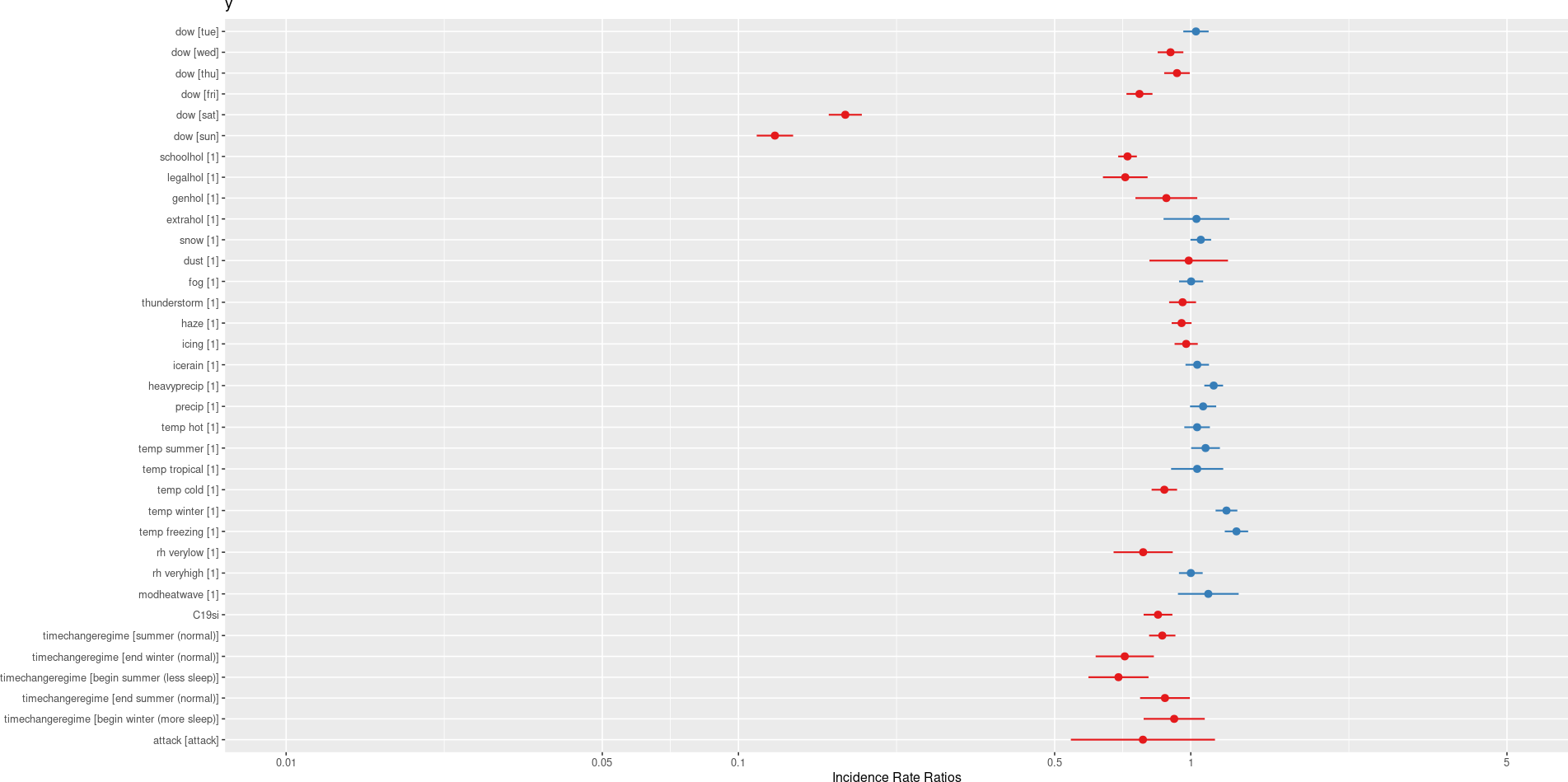
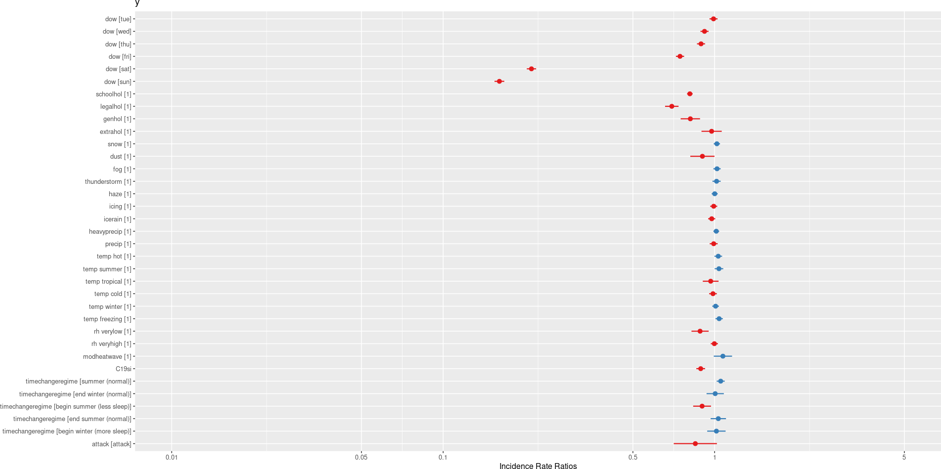
Both models are shown side-by-side in Figure 3.219 for easier comparison. Overall, the temporal patterns for commuting and workplace OA are quite similar, with both models showing significant reductions on weekends and holidays. However, some differences are noted, such as the more pronounced effect of legal holidays on workplace accidents compared to commuting accidents. Weather-related factors also appear to have a stronger influence on commuting accidents. These findings suggest that while general temporal trends are consistent across both types of OA, specific factors may differentially impact commuting versus workplace incidents.
Both models incorporate the same set of predictors, including day-of-week effects, holiday indicators, extreme weather condition indicators, COVID-19 stringency index (C19si), time change regimes, and terrorist attacks. This consistency in predictor inclusion allows for a direct comparison of their effects across the two contexts. The IRR for weekdays show a similar decreasing trend from Tuesday to Sunday in both models, with the lowest IRR observed during the weekend, indicating reduced activity levels. Similarly, legal and school holidays are associated with significantly lower OA numbers in both commuting and workplace settings, suggesting a general reduction in mobility during these periods.
However, the models differ in their explanatory power and the statistical significance of certain predictors. The workplace OA model shows a substantially higher R² value (0.945) compared to the commuting OA model (0.703), indicating that it explains a greater proportion of variance in the outcome (number of accidents). This suggests that workplace OA numbers are more systematically influenced by the included predictors -possibly due to more structured behavioural patterns in work environments- whereas commuting may be more variable and shaped by personal choices. Although some temporal patterns may exert more systematic influence in the workplace model, their effects appear less pronounced, as the IRRs in the workplace model are generally closer to 1.
Differences also emerge in the significance levels of specific predictors. For instance, freezing conditions have a stronger effect in the commuting model (IRR = 1.26, p < 0.001) than in the workplace model (IRR = 1.04, p = 0.017), suggesting that abnormal cold may influence commuting accidents more than workplace accidents. The COVID-19 stringency index (C19si) is significant in both models, but again with slightly stronger effects in the commuting context (IRR = 0.85 in the commuting vs. 0.89 in the workplace model), potentially reflecting greater sensitivity of commuting patterns to public health restrictions. For the summer hour period as a whole (excluding the weeks before and after the time changes), the effect even appears to be opposite: a small but significant decrease in commuting OA numbers (IRR = 0.86, p < 0.001) versus a small but significant increase in workplace OA numbers (IRR = 1.05, p = 0.003).

Temporal patterns in commuting and workplace occupational accidents
- Fewer occupational accidents on weekends and holidays. Both commuting and workplace accidents drop significantly on Saturdays, Sundays, and during school/legal holidays—reflecting reduced activity on these days.
- Weather matters more for commuting occupational accidents. Harsh weather (like snow or freezing temperatures) increases commuting accidents more than workplace ones.
- COVID-19 restrictions lowered all occupational accidents. Stricter COVID-19 measures were linked to fewer accidents, especially for commuting.
- No evidence for negative impact of time changes from our analysis. Shifts to and from daylight saving time showed no clear link to more occupational accidents.
3.5 Multivariable analysis of potential determinants
3.5.1 Likelihood to notify an OA (hadOA, model 1)
In this first multilevel logistic multivariable regression model, we examine the factors associated with the likelihood that an individual working in a company reports an OA in a given month during the ten-year study period (hadOA).
The model comprises 7,938,537 monthly observations (coded as 0 for no OA notified and 1 for an OA notified for a given individual in a given month), covering 291,661 unique individuals across 16,362 mutual ESPP/PS companies for which complete information on all model determinants is available.
Overall, 31,822 notifications are counted (out of total of 7,938,537 observations), corresponding to an overall monthly reporting probability of 0.4% per individual.
The model includes both fixed effects (individual and company level predictors) and random effects (group-level variation across companies and individual clusters in time) and explains a substantial portion of the variance, with a marginal R² of 0.136 and a conditional R² of 0.328. This indicates that both individual and group-level factors contribute meaningfully to the outcome. The random intercepts show that group level heterogeneity lies with individuals (individual variance = 0.76) as well as between companies (company variance = 0.19). The estimated ICC was 0.22. This result suggests that 22% of the variance is attributable to differences between individuals and between companies. Since the ICC is much larger than 0.10, the use of a multilevel approach is justified (Section 3.2.2.2). Properties and random effects of the full multivariable model (right) in comparison with the corresponding null model (left) are presented in Figure 3.220. Fixed effects estimates of the multivariable full model in comparison the corresponding univariable models and existing literature are shown in Figure 3.221.
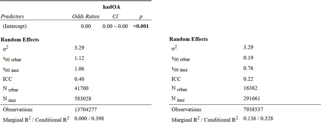
Significant determinants identified in the multivariable regression model, confirming the results of the corresponding univariable regression models, are ranked using the univariable regression model’s highest marginal/conditional R² ratios and reported with their multivariable regression Odds Ratio (OR).
Determinants associated with the likelihood of reporting an OA include the following.
- Salary level. Wage categories were strongly associated with the odds of reporting an OA. Compared to the reference group earning less than <€50 per day, the highest odds were observed in the €100–124 bracket (OR = 4.44) with a gradual decline towards the highest wage category (\(\geq\) €250, OR = 2.43). Although the magnitude differs, our findings support the work of Cabrera-Flores et al. (2023), which found that among Peruvian industries between 2016 and 2021, a 10% increase in average wages was associated with a 19% decrease in the rate of work accidents. Additionally, systematic reviews and empirical studies consistently show that low-wage workers are more likely to underreport workplace injuries and illnesses. Barriers include fear of retaliation, job loss, or reduced hours, as well as lack of knowledge about reporting procedures and perceptions that injuries are “part of the job” (Gholamizadeh et al., 2023; Mudenha et al., 2022). This might explain the discrepancy of the high estimates of all categories compared to the reference category. Alternatively, the theory that higher wages may reflect compensation for increased job risk could also be relevant (Lalive, Rafael and Ruf, Oliver and Zweimuller, Josef, 2006). See Section 1.3.2.5 and Section 3.4.1.5.
- Sector. Compared to the agriculture, forestry and fishing reference category (level A), only construction (level F) and human health and social work activities (level Q) show a significant higher likelihood of reporting an OA, with odds ratios of OR=1.31 and OR=1.28, respectively. In contrast, accommodation and food service activities (OR=0.49) and information and communication (OR=0.53), levels I and J, show significantly lower odds of reporting an OA. The higher odds for sector levels F and Q are in line with the high incidence rates reported by Eurostat. See Section 1.3.5 and Section 3.4.4.
- Workforce segment. Employees with white-collar status had substantially lower odds for reporting an OA (OR = 0.47). This is in line with expectations and former research. See Section 1.3.3.1 and Section 3.4.2.1.
- Biological sex. Men were more likely than women to report an OA (OR = 1.18), confirming findings from former studies on the topic. See Section 1.3.2.2 and Section 3.4.1.2.
- Insurance companies. The model reveals significant differences in the likelihood of reporting an OA, depending on the insurer. The odds ratios range from 0.93 to1.37. This suggests that the insurer may play a role in the reporting behaviour and/or notification process. This could reflect differences in how insurers communicate with employers and workers, or facilitate the reporting process. We could hypothesize for example that some insurers may have more proactive procedures, better digital infrastructure, or promote stronger safety cultures that encourage reporting. As this is a novel observation, it warrants further investigation to confirm and explain the underlying mechanisms. See Section 1.3.4.4 and Section 3.4.3.5.
- Age. Individuals aged 20–59 had significantly higher odds of reporting an OA compared to the reference group (under 20), with the highest odds observed among workers aged 20-29 (OR = 1.27). This confirms the commonly observed trend that younger workers are more likely to experience OAs. See Section 1.3.2.1 and Section 3.4.1.1.
- Nature of the contract. Full-time workers had significantly higher odds of reporting an OA (OR = 1.39) which confirms previous literature on the topic. See Section 1.3.3.3 and Section 3.4.2.3.
- Work experience. Longer work experience was associated with lower odds of reporting an OA, showing a decreasing trend from 1–4 years (OR = 0.94) to \(\geq\) 21 years (OR = 0.69). In this study, work experience is defined as the duration of the employment contract with the current employer which may relfect a mix of job-specific and employer specific experience, but not overall career experience. These findings are consistent with former research stating that lower job experience correlates with a higher likelihood of OA. See Section 1.3.2.3 and Section 3.4.1.3.
- Company size. Larger companies (\(\geq\) 200 employees) were associated with significantly higher odds of OA occurrence (OR = 1.70) in the univariable model, compared to the reference group (<5 employees). However, this pattern was reversed in the multivariable model, which revealed a more nuanced relationship. Companies with up to 49 employees showed decreasing odds ratios, confirming earlier findings that smaller companies tend to report relatively more OAs. Between 50 and 200 employees, the odds ratios increased, approaching the level of the reference group, and continued to rise beyond 200 employees. This shift suggests a complex organisational effect, likely influenced by confounding factors such as sector, which are accounted for in the multivariable model. The discrepancy between the univariable and multivariable results highlights the importance of adjusting for such determinants. While the univariable model presents a straightforward positive association with company size, the multivariable analysis uncovers a negative relationship up to 50 employees, followed by a reversal in the higher brackets. These findings align with previous research and underscore the multifaceted nature of the relationship between company size and OA occurrence. See Section 1.3.4.2 and Section 3.4.3.2.
- Work location. Certain Belgian provinces such as Limburg, Namur, East Flanders, and West Flanders showed significantly higher odds, compared to the reference province Antwerp. In contrast, Brussels and Hainaut did not show significantly higher odds. While the overall pattern in the multivariable model is similar to the univariable model, confidence intervals tend to be wider than those of other determinants. Additionally, the low univariable R² ratio of 1% (0.004/0.405) suggests that variation in the geographic location of the employer has only a limited impact on the model’s overall explanatory power. See Section 1.3.4.1 and Section 3.4.3.1.
- Temporal effects. The likelihood to report an OA in 2023 remains still significantly lower than in 2014. While there was adeclining trend from 2014 to 2019, this pattern reverted in recent years (2020–2023). Across all years, reporting likelihoods also varied by month. Compared to January, the odds for reporting OAs were significantly lower in all months (except March, June, September and October). See Section 1.3.6 and Section 3.4.5.
The multivariable model highlights that individual demographic characteristics (age, gender), employment conditions (wage, experience, company size), and temporal factors (year and month) are significant determinants of reporting an OA. The effects of wage and company size suggest that structural and economic factors play a critical role, while the temporal decline may reflect broader labour market trends or policy changes.
Wage, sector and workforce segment, but also biological sex and insurer play an import role in notification patterns of occupational accidents
The multivariable model demonstrates substantial explanatory power for predicting the notification of an occupational accident. Wage, sector, and workforce segment show the highest marginal-to-conditional R² proportions in their respective univariable models, closely followed by biological sex and insurer. The model highlights the importance of accounting for both individual- and company-level variation when attempting to explain the likelihood of reporting an occupational accident.
Figure 3.221 shows the different effect sizes of the categories included in the model. The figure immediately indicates large effects for wage, workforce segment and sector since their estimates (dots with whiskers) lie relatively further from the OR=1 reference line compared to the other variables included in the model.
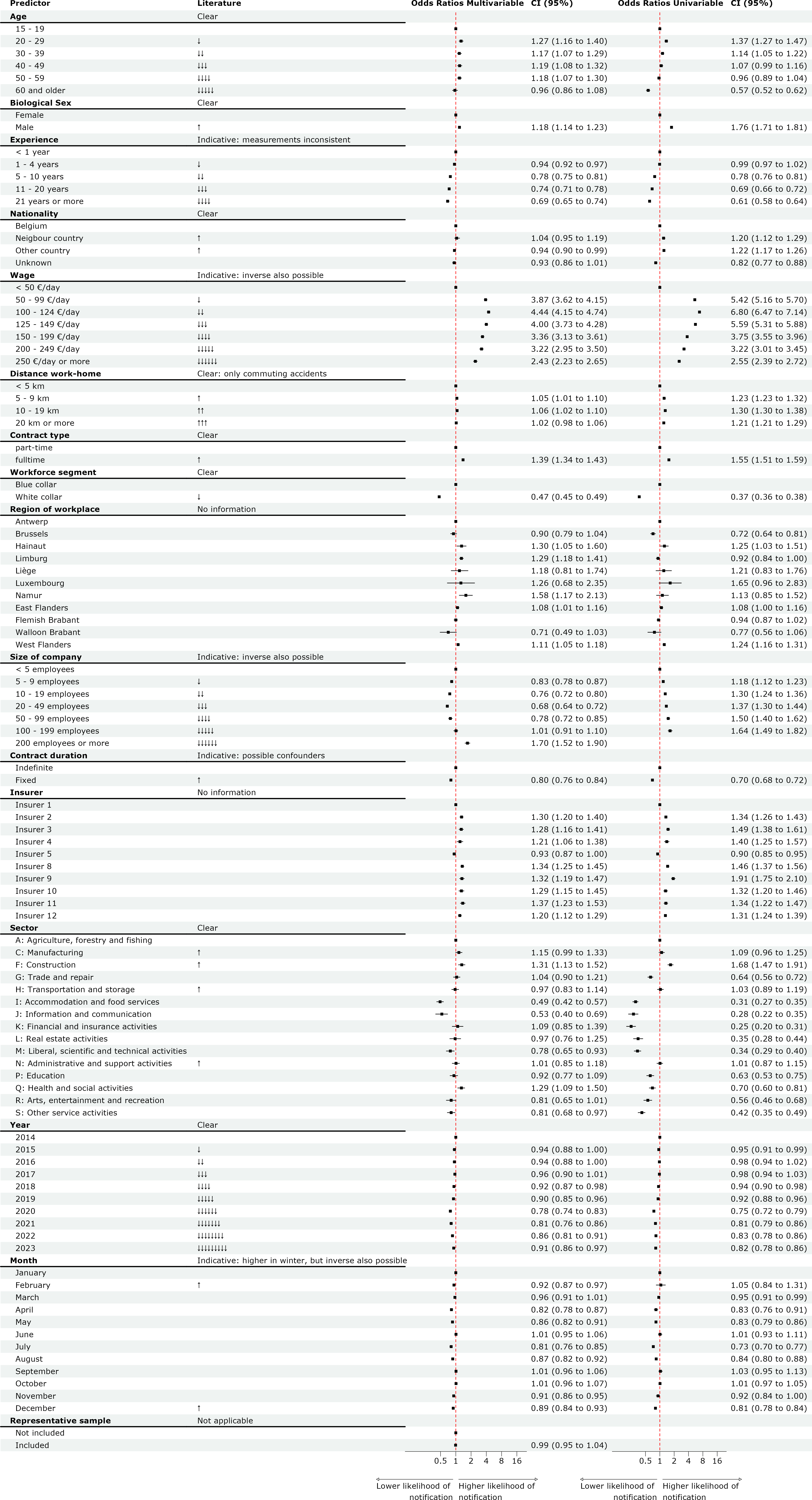
3.5.2 Likelihood to refuse an OA (statusOA, model 1.1)
This multilevel logistic multivariable regression model estimates the probability that a reported OA is refused by an OA insurer in a given month during the ten-year study period (statusOA).
The model comprises 31,645 observations or notifications of single OA (coded as 0 for a not refused OA and 1 for a refused OA), across 25,200 unique individuals and 7,218 mutual ESPP/PS companies for which complete information on all model determinants is available.
Overall, 2,797 refusals are counted out of 31,645 observations, indicating an overall refusal rate of 8.8%. This is somewhat lower as the figures reported in FEDRIS’ year report 2023 Fig 1.2b -for the private sector- ranging from 10.6% in 2014 to 16.2.3% in 2023 (Federal Agency for Occupational Risks, 2023).
The model includes fixed effects for a wide range of individual (victim-level) and collective (company-level) variables, as well as random effects for both individuals (personal identification number within NSSO (INSZ number) (insznr)) and companies (enterprise identification number within CBE (crbnr)). The variable pseudins refers to a pseudonymized identifier of an OA insurer and is included as a fixed effect, reflecting the limited and predefined group of 13 OA insurers in Belgium. Of these, 10 are included in the model. The remaining three were excluded due to either an insufficient number of cases in certain category combinations or a high proportion of unknown decisions (data not shown).
The random effect variance for individuals (insznr) is high (\(\tau_{00\,\text{insz}}\) = 329.80), indicating substantial unexplained heterogeneity at the individual level. Although the company-level variance is near zero (\(\tau_{00\,\text{crbnr}}\) = 0.00), suggesting that company affiliation does not contribute meaningfully to the likelihood of refusal by an insurer, we retain the clustering to respect the data’s hierarchical structure and ensure accurate standard error estimation.
The model shows a conditional R² of 0.990, indicating that nearly all variation in refusal outcomes is explained when both fixed and random effects are considered. However, the marginal R² is only 0.001, showing that the fixed effects, such as insurer identity, contribute virtually nothing in explaining the outcome of refusal. This suggests that the model’s explanatory power lies almost entirely in the between-individual variation, with the individual-level random effects accounting for nearly all of the explained variance. Properties and random effects of the full multivariable model (right) in comparison with the corresponding null model (left) are presented in Figure 3.222. Fixed effects estimates of the multivariable full model in comparison the corresponding univariable models and existing literature are shown in Figure 3.223.
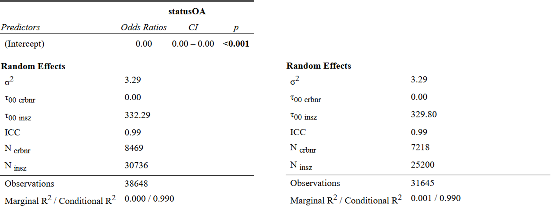
The indications of slightly higher refusal chances for part-time workers (see Section 3.4.2.3) or workers in the company segment of 100 to 199 employees (see Section 3.4.3.2), or a lower refusal chance for insurer 9 (see Section 3.4.3.5), do not withhold in the multivariable model after correction for all other potential determinants.
Although the fixed effects for insurers (pseudins) show some variation in odds ratios (4, 2 and 9 somewhat lower versus 11 and 12 somewhat higher), none of these effects reach statistical significance. This means that -while differences in refusal behaviour still may occur- the model does not suggest any significant systematic insurer-level bias.
The model includes over 100 categorical levels, yet only one (the year 2017) appears statistically significant at the conventional 5% level. However, without correcting for multiple testing, this result may be misleading. With so many tests, it is statistically expected that around five categories could appear significant purely by chance. Therefore, the observed effect for 2017, although consistent with a broader trend of lower refusal rates between 2016 and 2017, may represent a false positive. Since our study does not cover the public sector, we cannot confirm the decreasing trend from 2020 on for the public sector shown in the FEDRIS year report 2023 Fig 1.2b (Federal Agency for Occupational Risks, 2023), but with our model showing a rather increasing trend from 2017 on, we can confirm the FEDRIS results for the private sector.
Since the model primarily includes demographic and employment-related variables (e.g. age, wage, nationality, company size) and lacks information on the circumstances of the accident itself (such as severity, type, or claim completeness, delay between the moment of the accident and it’s notification,…) it has only very limited ability to explain refusal decisions. This limitation reflects the model’s scope rather than a flaw, and suggests that refusals may be more closely tied to accident-specific or procedural factors not captured here.
Without inclusion of occupational accident specific determinants and procedural factors, no significant determinants for refusals are found
The model demonstrates strong fit at the individual level but weak explanatory power from fixed effects, including insurer identity. The dominant source of variation is individual-level heterogeneity, with company affiliation playing no measurable role. The model’s utility for identifying systematic refusal patterns is limited by the absence of occupational accident specific variables. Like for all other determinants included in the model, with exception of the year 2017, no significant differences in refusal patterns between insurers are noticed.
Figure 3.223 shows that the studied set of variables does not significantly determine whether an insurer accepts or rejects an OA claim. Hence, the model does not show indications of discrimination in insurance decisions, nor significant differences in refusal chances between insurers.
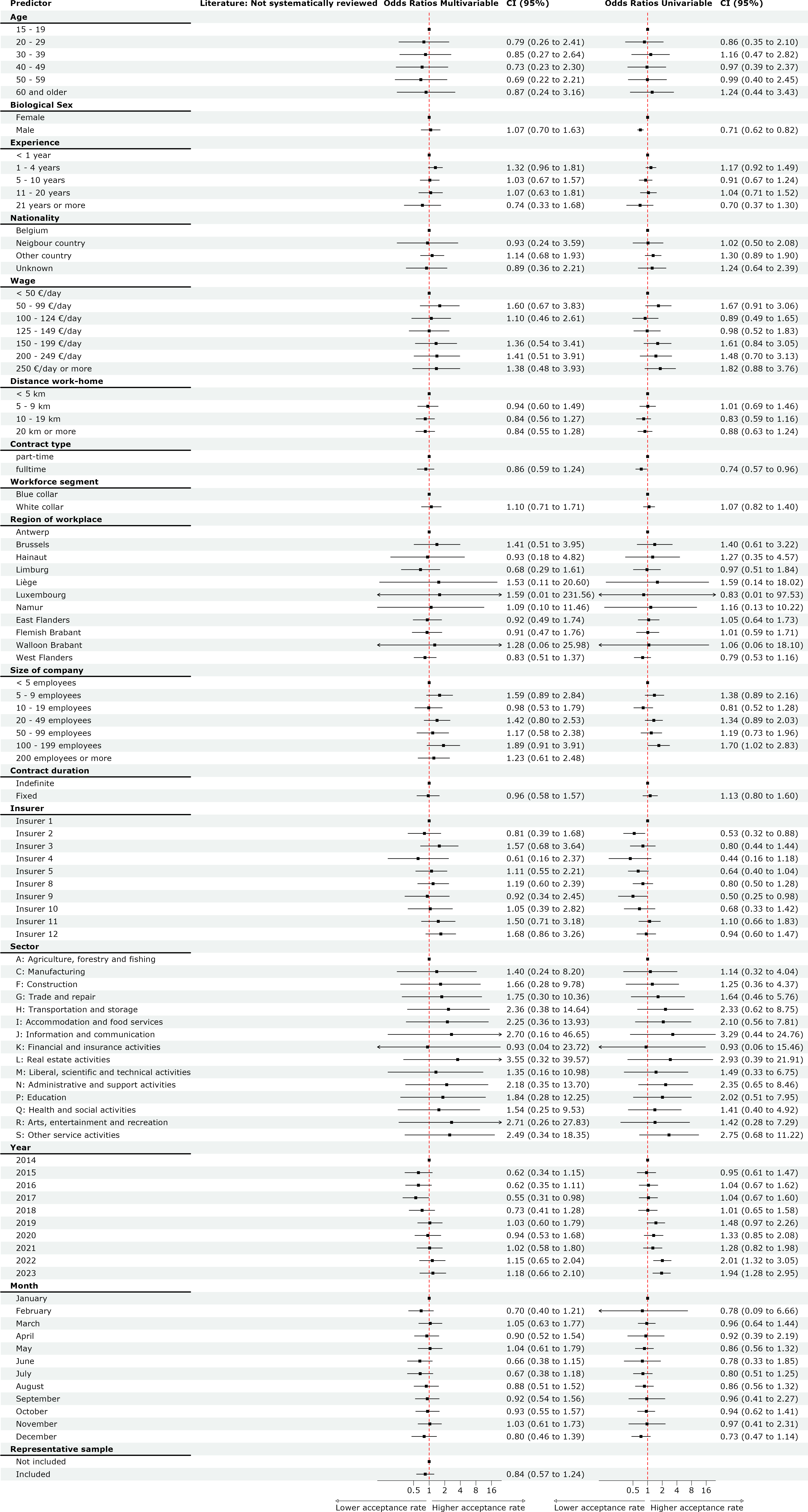
Potentential for further investigation
Some procedural accident meta variables (see Section 2.8.1.2) currently not included in the model may be worth further investigation. Examples include the time between the occupational accident and the first declaration to the insurer, the number of notifications, the similarity degree between multiple notifications, whether serious accidents were investigated within ten days after occurrence,…
3.5.3 Likelihood to experience an accepted commuting OA (comOA, model 2)
This multilevel logistic multivariable regression model estimates the probability of an insurer-accepted commuting OA (comOA) in a certain month during the ten-year study and explores the associated risk factors.
The model includes 7,938,537 monthly observations (0 no accepted commuting OA, 1 an accepted commuting OA for a given individual in a certain month), across 291,661 unique individuals and 16,362 mutual ESPP/PS companies for which information on all determinants included in the model is available.
Overall, 4,182 accepted commuting OA are counted under the whole of 7,938,537 observations, which implies an overall individual chance on an accepted commuting OA in a certain month of 0,1%. On a total of 28,848 accepted OA, the commuting accidents represent 14,5% of all accepted OA in our dataset.
The model includes fixed effects for individual- and company-level predictors and random effects to account for variation across individuals and companies over time. The random intercepts show that nearly all unexplained heterogeneity lies between individuals (individual variance = 52.45) rather than between companies (company variance = 0.00), resulting in an estimated ICC of approximately 0.94. Fixed covariates alone explain about 18.3% of the variance, while adding individual-level random intercepts increases the explained variance up to 94.6% (inferred from the null model since the conditional R² could not be calculated directly for the multivariable model), indicating strong person-specific baseline propensities for experiencing commuting OA. Properties and random effects of the full multivariable model (right) in comparison with the corresponding null model (left) are presented in Figure 3.224. Fixed effects estimates of the multivariable full model in comparison the corresponding univariable models and existing literature are shown in Figure 3.225.
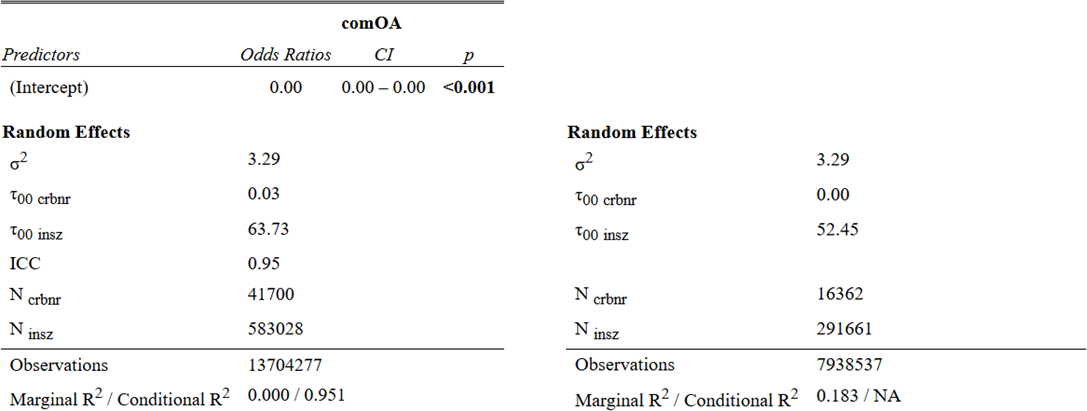
Significant determinants identified in the multivariable regression model, confirming the results of the corresponding univariable regression models, are ranked using the univariable regression model’s highest marginal/conditional R² ratios and reported with their multivariable regression OR.
Determinants of an insurer-accepted commuting OA include the following.
- Salary level. Wage categories were associated with odds of an insurer-accepted commuting OA; compared to the reference category of <50 euro day wage, odds were highest in the 50-99 bracket (OR = 8.67) and gradually decreased towards the highest bracket (\(\geq\) 250, OR = 5.05. The discrepancy of the high estimates of all categories in comparison to the reference category of <50 needs further investigation. See Section 1.3.2.5 and Section 3.4.1.5.
- Insurancy companies. 5 lowest (OR = 0.88), 8 highest (OR = 1.36). This suggests that differences between OA insurers in some way might affect the likelihood on an insurer accepted commuting accident. This is a new finding that needs confirmation in future studies. See Section 1.3.4.4 and Section 3.4.3.5.
- Temporal effects. The model reveals seasonal variation with the highest relative risk in the January reference category and much lower odds in July (OR = 0.42) and August (OR = 0.50). Significantly elevated odds occur in 2017, 2022 and 2023 and a clear trend of increasing odds is apparent from 2020 (the Corona-crisis induced a steep drop in commuting displacements) to 2023. This year trend likely reflects a broader mobility trend rather than company-level changes (Assuralia, 2025b, 2025a). This pattern may be observed due to changes in commuting habits, such as the growing use of bicycles, differences in workforce composition, reporting practices, or operational characteristics such altering work patterns with a potential impact on commuting patterns. See Section 1.3.6 and Section 3.4.5.
- Work experience. Longer work experience was associated with lower odds on an insurer-accepted commuting OA, with a decreasing trend from 1–4 years (OR = 0.87) to \(\geq\) 21 years (OR = 0.70). Tt is unclear how job or employer specific work experience would be related to commuting accidents. One possible explanation is that work experience may be acting as a proxy for younger drivers who are known to be at higher risk in traffic incidents. The current age categories may be too broad to capture this nuance, whereas the tenure variable -especially the “less than one year” category- might better reflect the elevated risk among young and inexperienced commuters. Future research could benefit from refining age categorization (e.g., isolating the 18–24 group) and comparing it more directly with tenure to disentangle experience from age-related risk. See Section 1.3.2.3 and Section 3.4.1.3.
- Nature of work. Full-time workers had significantly higher odds (OR = 1.26). See Section 1.3.3.3 and Section 3.4.2.3.
Distance to work does not appear to influence risk after adjustment, but this does not rule out differences by mode of transport, which could not be included in the model. Like demonstrated in other reports, adding information on commuting mode could provide clearer insights (Assuralia, 2025b, 2025a). See Section 1.3.2.7 and Section 3.4.1.7.
The same applies to biological sex. After adjustment in the multivariable model, the previously significant association -suggesting that men experience significantly fewer commuting-related OAs- no longer holds. It is important to note that findings from other studies, such as the Medex study (Federal Public Service Health, Food Chain Safety and Environment, 2022), are often based on univariable analyses and limited to the subset of workers who have experienced (commuting) OAs. Additionally, previous research has highlighted that women are underrepresented as drivers and passengers in cars (VIAS Institute, 2018), which may influence observed patterns. While future studies may again identify a statistically significant effect of biological sex, we anticipate that both the effect sizes and the practical relevance of sex as a determinant of commuting-related OAs will remain limited. See Section 1.3.2.2 and Section 3.4.1.2.
In the present study, no evidence was found to support that age would be a key determinant of the likelihood of experiencing an accepted commuting accident. Previous research has reported higher incidence rates among older workers, particularly those aged 45–65, compared to younger age groups. However, the pattern observed in our data -although not statistically significant- suggested a decreasing rather than increasing trend between ages 20 and 60. Earlier studies have also examined the interaction between age and biological sex, indicating that older women may be especially vulnerable to commuting accidents, while older men are more frequently involved in work-related traffic accidents during working hours (Delgado-Fernández et al., 2022; Nenonen, 2011; Salminen, 2000). This interaction was not explored in the present study. See Section 1.3.2.1 and Section 3.4.1.1.
Limited impact of sex and age when other factors are considered
Although previous studies often identified biological sex and age as important risk factors for commuting accidents, our findings suggest their influence is relatively minor when other factors are considered across a broader worker population. We conclude that being male or older does not substantially increase or decrease the likelihood of experiencing a commuting occupational accident once additional variables within the exposed population are taken into account.
In 2017, Belgium experienced a relative increase in the number of traffic accidents occurring during commuting (home-to-work travel), as reported by the VIAS institute. This rise was notable despite a general decline in overall traffic fatalities and injury-related accidents, suggesting that commuting incidents constituted a proportionally larger share of total traffic accidents that year. Several contributing factors were identified, including increased mobility, longer commuting distances, the growing use of alternative transport modes such as bicycles and electric scooters, and improved reporting mechanisms for traffic OA. However, data from 2018 indicate that this upward trend was not sustained. The VIAS institute’s 2018 Traffic Safety Barometer, reported a continued decline in traffic fatalities and a moderate decrease in the share of commuting-related accidents, implying that the spike observed in 2017 may have been influenced by temporary or situational factors rather than representing a structural shift.
Overall, the individual and company-level variables included in the model have limited explanatory power compared to the strong influence of individual-level heterogeneity. These results imply that prevention strategies should focus on person-level factors rather than broad company-wide measures.
Companies however can play a valuable role in targeted risk communication. Young aged (and/or early-tenure, see higher) and full-time employees represent different risk groups, and interventions should account for seasonal patterns, with increased efforts during winter and early spring. Large firms may warrant commuting-risk audits despite negligible random company effects, as fixed effects suggest meaningful differences in exposure and reporting contexts. Distance alone is not informative, so future analyses incorporating commuting mode and exposure measures could improve interpretability and actionability.
Individual-level heterogeneity is more important in explaining insurer-accepted commuting occupational accidents over wage, time and some other fixed effects
Our research shows that the risk of having an insurer-accepted commuting accident depends much more on personal differences between individuals than on factors like salary, time of year, or other characteristics. This means that some people are simply more likely to have such accidents, regardless of where they work or how much they earn. As a result, prevention efforts should focus more on individual risk factors rather than on broad company-wide measures. Companies however can play a valuable role in targeted risk communication e.g. focusing on different risk groups with increased efforts in winter and early spring.
Figure 3.225 illustrates some significant differences for wage, insurer, month,… however, since individual risk appears to be substantially more influential than differences between companies, the observed effects should be interpreted with caution.
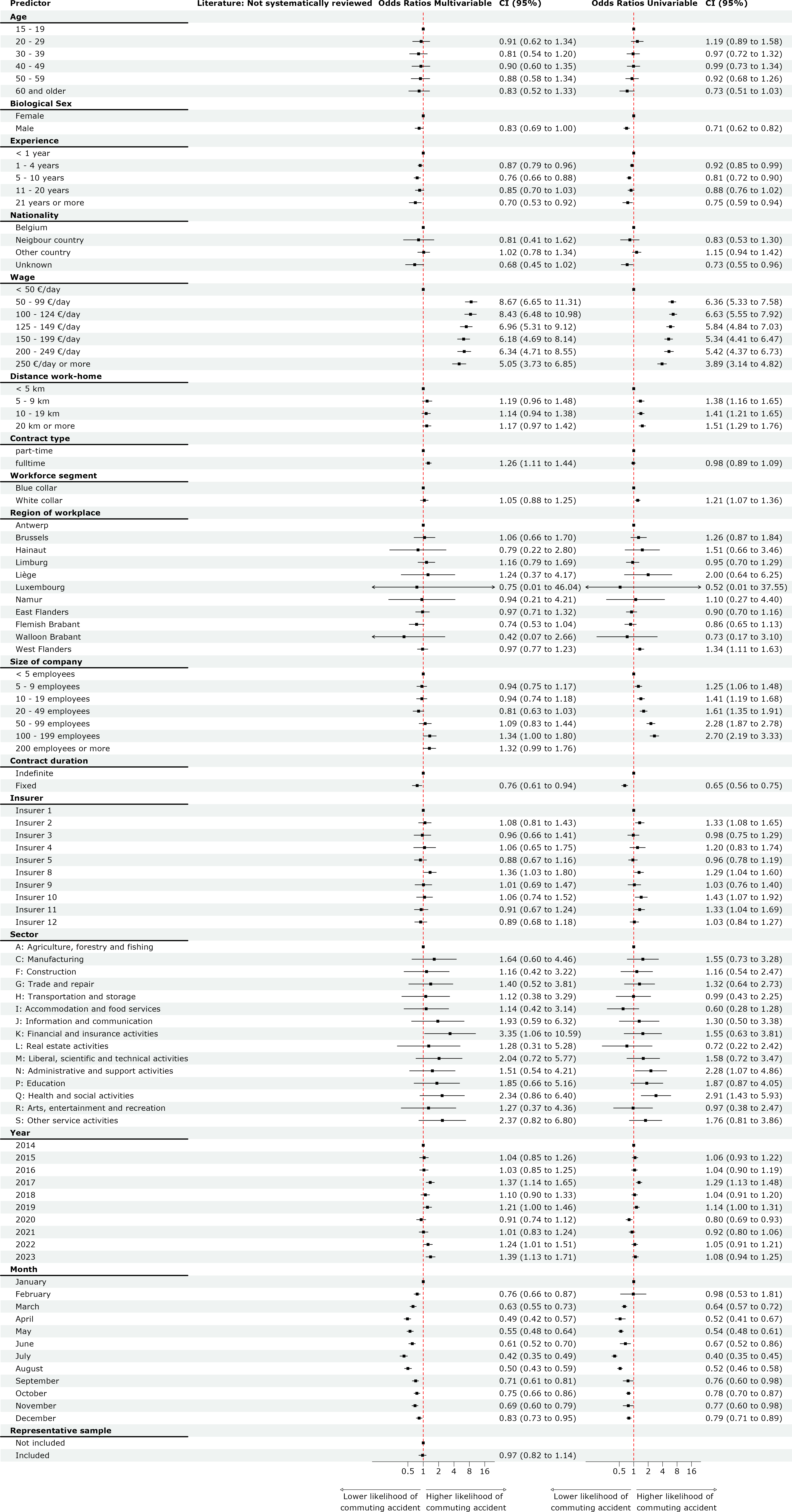
3.5.4 Likelihood to experience an accepted workplace OA (wplOA, model 3)
This multilevel logistic multivariable regression model estimates the probability of an insurer-accepted workplace OA (wplOA) in a certain month during the ten-year study and explores the associated risk factors.
The model includes 7,938,537 monthly observations (0 no accepted workplace OA, 1 an accepted workplace OA for a given individual in a certain month), across 291,661 unique individuals and 16,362 mutual ESPP/PS companies for which information on all determinants included in the model is available.
Overall, 24,666 accepted workplace OA are counted under the whole of 7,938,537 observations, which implies an overall individual chance on an insurer-accepted workplace OA in a certain month of 0.3%. On a total of 28,848 accepted OA, the workplace accidents represent 85.5% of all accepted OA in our dataset.
The model includes fixed effects at the individual and company level over time and random intercepts for persons and firms. The random effects indicate substantial heterogeneity at both levels (company variance = 0.20; individual variance = 0.91), with an ICC of approximately 0.25. Since the ICC is much larger than 0.10, the use of a multilevel approach is justified (Section 3.2.2.2). Fixed covariates explain 14.6% of the variance, while the full model (fixed plus random effects) explains 36.1%, suggesting that both observed characteristics and unmeasured person- or firm-level factors contribute more or less equally to variation in risk. This is in strong contrast with the results of the previously discussed model on commuting OAs. Properties and random effects of the full multivariable model (right) in comparison with the corresponding null model (left) are presented in Figure 3.226. Fixed effects estimates of the multivariable full model in comparison the corresponding univariable models and existing literature are shown in Figure 3.227.
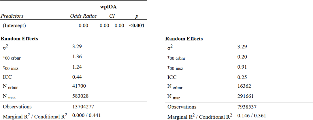
Significant determinants identified in the multivariable regression model, confirming the results of the corresponding univariable regression models, are ranked using the univariable regression model’s highest marginal/conditional R² ratios and reported with their multivariable regression OR.
Several individual characteristics are associated with the outcome. In the univariable models, wage (17%) and workforce class (13%) showed the highest marginal-to-conditional R² ratios, followed by sex (5%) and age (2%). Nature of contract, experience, and distance also explained some variance, but their ratios were close to 1% or less. Individual level determinants of an insurer-accepted workplace OA include the following.
- Salary level. Daily wage (in euros) is strongly associated with higher odds across wage bands compared with the lowest reference. Although the effect decreases at the highest bands (e.g., 50–99 OR = 3.67; 100–124 OR = 4.42; \(\geq\) 250 OR = 2.42). See Section 1.3.2.5 and Section 3.4.1.5.
- Workforce segment. White-collar employees (bedienden) have substantially lower odds (OR = 0.41) compared with blue-collar workers (arbeiders). See Section 1.3.3.1 and Section 3.4.2.1.
- Biological sex. Men have higher odds than women (OR = 1.27). See Section 1.3.2.2 and Section 3.4.1.2.
- Age. Compared with the reference age group, workers aged 20–59 show increased odds (e.g., 20–29 OR = 1.41; 30–39 OR = 1.27; 40–49 OR = 1.29; 50–59 OR = 1.28), while those aged 60+ do not differ significantly. See Section 1.3.2.1 and Section 3.4.1.1.
- Nature of the contract. Full-time contracts are associated with higher odds (OR = 1.40). See Section 1.3.3.3 and Section 3.4.2.3.
- Contract type. Limited-duration contracts show lower odds (OR = 0.82). See Section 1.3.3.2 and Section 3.4.2.2.
- Work experience. Tenure within the current employer is protective, with progressively lower odds at longer tenures (1–4 years OR = 0.96; 5–10 years OR = 0.80; 11–20 years OR = 0.75; \(\geq\) 21 years OR = 0.72). See Section 1.3.2.3 and Section 3.4.1.3.
- Commuting distance. Distance to work shows only minor associations (10–19 km OR = 1.07). See Section 1.3.2.7 and Section 3.4.1.7.
Company and contextual characteristics also influence the likelihood. In univariable models, NACE-BEL 2008 sector and insurer fixed effects showed high marginal-to-conditional R² ratios (14% and 4%, respectively). Company-level determinants of an insurer-accepted workplace OA include the following.
- Sector. Several NACE-BEL 2008 sections have lower odds compared with the reference (e.g., I OR = 0.42; J OR = 0.26; K OR = 0.64; M OR = 0.57; R OR = 0.67; S OR = 0.56), while section F (construction, OR=1.25) and Q (human health and social work activities care, OR=1.21) are the only sectors with a higher likelihood compared to agriculture, forestry an and fishing (level A). See Section 1.3.5 and Section 3.4.4.
- Insurance companies. Insurer category (pseudins) also matters, some categories show higher odds (e.g., 9 and 11 OR = 1.31) and others lower (e.g. 5 OR = 0.92). See Section 1.3.4.4 and Section 3.4.3.5.
- Work location. Geographic location of the employer. Some provinces have higher odds (e.g., Limburg OR = 1.46; Namur OR = 1.83; West Flanders OR = 1.15), others lower (e.g., Brussels OR = 0.80), while several show no meaningful difference. See Section 1.3.4.1 and Section 3.4.3.1.
- Company size. Odds are lower for firms with 5–49 employees (OR 0.75 to 0.82), similar for 50–99, and substantially higher for larger firms (100–199 OR = 2.36; \(\geq\) 200 OR = 17.68) compared with the smallest reference group. See Section 1.3.4.2 and Section 3.4.3.2.
And finally, also time level effects seem to contribute to the risk. In univariable models, year and month fixed effects showed small but significant effects that could be confirmed in the multivariable model. Time-level determinants of an insurer-accepted workplace OA include the following.
- Year. Over time, odds are generally lower than in the baseline year, with a marked reduction from 2020 onwards but showing a slightly increasing trend (2020 OR = 0.77 to 2023 OR = 0.84). See Section 1.3.6 and Section 3.4.5.
- Month. Seasonal variation is present, with several months (April, May, July and December) below January levels and slightly elevated odds in June (OR = 1.09), September and October (OR = 1.08). See Section 1.3.6 and Section 3.4.5.
Overall, these findings indicate higher risk among men, younger to middle-aged workers, those on full-time contracts, and employees in very large firms, and lower risk among those with longer tenure, white-collar status, certain sectors, and in many months and recent years compared with their respective reference categories.
Wage, workforce segment, sector, biological sex, and insurer influence workplace occupational accidents patterns
The multivariable model shows good explanatory power for accepted workplace occupational accidents. Wage, workforce segment, and sector contribute the most, as indicated by their high marginal-to-conditional R² proportions in the corresponding univariable models. Biological sex and insurer also play a notable role. Both individual-level and company-level heterogeneity are key drivers in the observed patterns.
Figure 3.227 displays the estimated effect sizes for each category included in the model. The figure clearly highlights substantial effects for wage, workforce segment, and sector, as their estimates (represented by dots with whiskers) are positioned further from the OR = 1 reference line compared to other variables, indicating stronger associations with accepted workplace accidents.
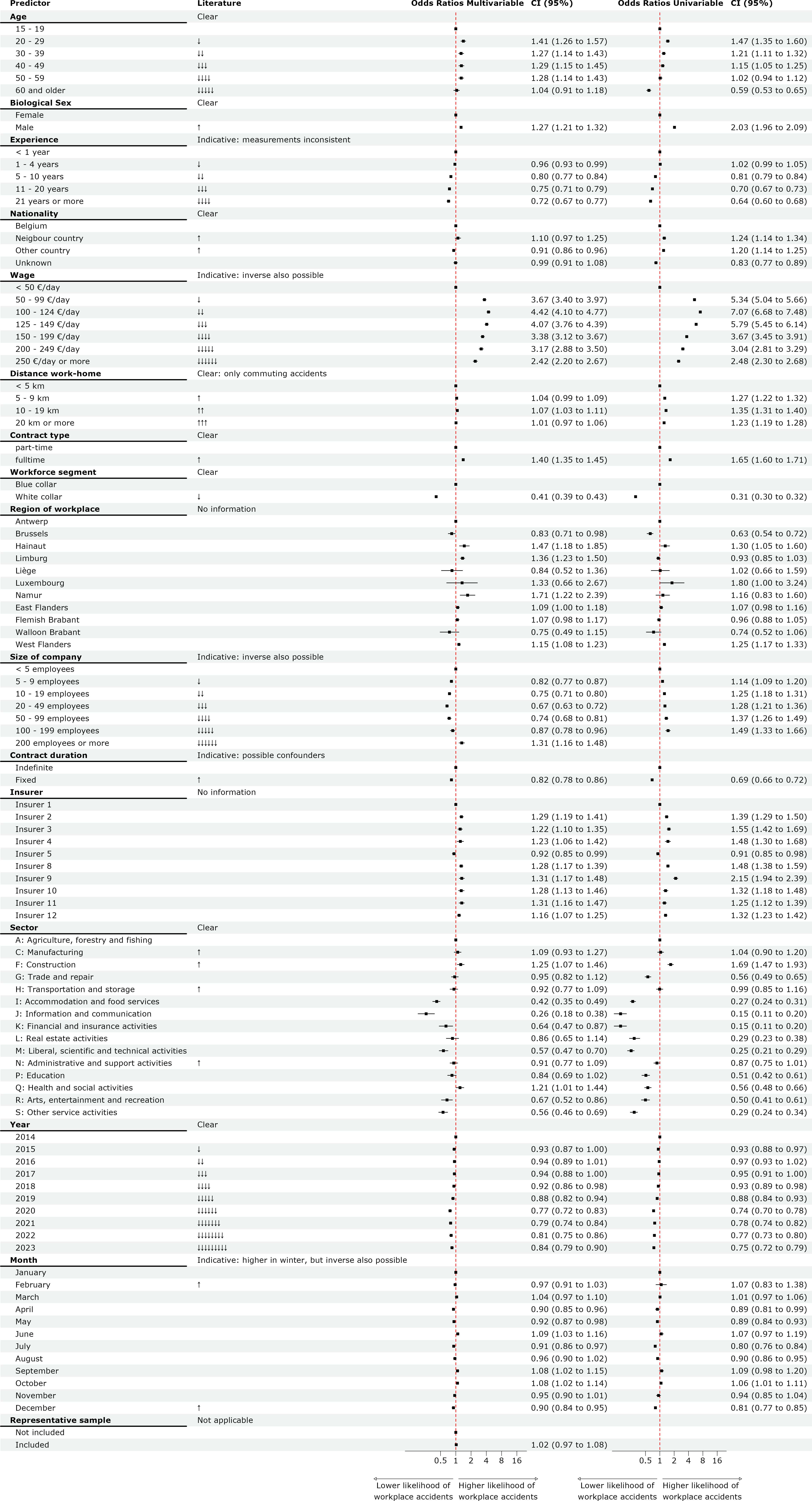
3.5.5 A number of reflections on our commuting and workplace accident models
Our findings indicate that, based on the variables included in the models, it is challenging to formulate targeted prevention policies that would consistently reduce accident rates. This difficulty is primarily due to the substantial influence of random effects, reflecting unmeasured heterogeneity at both the individual and company levels. For workplace accidents (wplOA, see Section 3.5.4), the random effect at the company level is particularly pronounced, suggesting that organisational context plays a significant role in shaping safety outcomes. In contrast, for commuting accidents (comOA, see Section 3.5.3), the company-level random effect is negligible, indicating that such incidents are less influenced by organisational characteristics.
Both models include a range of fixed effects at the individual and organisational levels. In Section 3.5.4, several predictors show strong associations with accident likelihood, including age, sex, tenure, employment status, company size, and sector. Younger workers, males, full-time employees and those with shorter tenure are more likely to experience workplace OA. Organisational characteristics such as large company size (\(\geq\) 200 employees) and high-risk sectors, particularly construction, also contribute significantly. In comOA, while some individual-level predictors such as tenure and employment status remain relevant, the overall explanatory power of the model is lower, and company-level characteristics have limited predictive value.
Temporal variables provide additional insights. From 2020 onward, both models show an increased likelihood for OA, probably reflecting changes in work patterns, reporting behaviour, or external conditions such as the COVID-19 pandemic. Clear seasonal trends also emerge: commuting accidents are more likely to occur between November and February, while workplace accidents show higher likelihoods in March, June, September, and October. These patterns suggest potential levers for organisations, such as adjusting work schedules, operational planning, or communication campaigns to align with periods of elevated risk.
Although distance to work is included as a variable in the commuting model, it does not emerge as a strong predictor. This suggests that other factors -such as mode of transport and timing of travel- may be more relevant. These factors are potentially modifiable through company policies, including flexible start times, telework arrangements, and mobility programs. While the statistical contribution of company-level variance in comOA is minimal, large firms may still be well-positioned to implement and scale commuting-related interventions.
The current models do not include data on specific preventive measures, such as safety training, engineering controls, or behavioural interventions. Consequently, their effectiveness cannot be evaluated within the scope of this analysis. This limitation highlights the need for a follow-up phase in which the random effects are explored in greater detail. Incorporating additional contextual information -such as the presence of safety campaigns, onboarding programs, or infrastructure investments- could help reduce the unexplained variance and allow for a more precise assessment of targeted interventions. However, collecting such data over a sufficiently long period remains a practical challenge.
Sectoral differences in OA risk are to be expected, but they also raise questions about how organisations manage risk. This relates to the concept of safety culture, which reflects the extent to which risk awareness and management is embedded in organisational practices. Although safety culture is inherently difficult to measure, potential proxies, such as near-miss reporting rates, or the frequency of supervisor safety conversations, may offer valuable insights. Future research should explore how such indicators can be integrated into predictive models.
A further avenue for investigation involves evaluating the impact of preventive measures over time. This could include assessing whether interventions such as training or workplace modifications lead to measurable reductions in accident rates within companies, and whether effective practices are adopted across similar organisations or sectors. Such analyses could help clarify the sector-wide impact of prevention strategies and support evidence-based policy development.
From a prioritization perspective, workplace safety (or prevention of workplace accidents) represents the most substantial and controllable opportunity for prevention advisors, particularly in large firms and high-risk sectors such as construction. Commuting safety (or prevention of commuting accidents), while less influenced by organisational context, remains a relevant area for targeted, policy-driven interventions. These are most effective when strategically aligned with seasonal risk patterns, early stages of employment, and company-level decisions regarding mobility and scheduling.
Keep the focus on workplace occupational accidents
Since around 85% of accepted occupational accidents are workplace-related (wplOA) and only about 15% are commuting-related (comOA), the most impactful and controllable opportunities for company-facing prevention advisors lie in addressing workplace accidents. ESPP prevention advisors work directly with companies, and because the largest share of accidents occurs in the workplace, focusing on wplOA stays more important than on commuting-relating accidents.
The multilevel model for workplace accidents also shows a strong signal between companies, suggesting that prevention advisors can make a difference by tailoring safety interventions to specific company profiles. This requires a strategic prioritizing and integration of layering measures that fit the company’s context and workforce characteristics.
It’s important to recognize that some factors influencing OAs are structural, such as wage level, tenure, contract type, and company size. While these elements fall outside the direct influence of prevention advisors, understanding their role is essential for the development of effective strategies. Conversely, modifiable factors such as experience and awareness and can be influenced through training, onboarding, mentoring, and seasonal safety campaigns.
Future research could aim to integrate more contextual and cultural variables to better understand and reduce the random effects that currently limit the predictive precision of the models.
Recognize structural components like low-wage, full-time and young workers in different company size segments and look for modifiable opportunities
For commuting accidents, seasonal campaigns, flexible work arrangements and transportation mode policies could help mitigate risks. For workplace accidents, targeted training, onboarding, mentoring, improved safety protocols and all other prevention measures fostering a strong safety culture could become key strategies. Prevention advisors are well-positioned to support organisations in addressing these modifiable factors, while also supporting them in remaining aware of the structural components that shape risk profiles.
3.5.6 Frequence degree of workplace OA (freqOA, model 4)
In this multilevel multivariable regression model we examine the factors associated with the company’s frequency degree in a given year during the ten-year study period (freqOA).
The model includes 81,780 yearly observations (frequency degree for a given company in a certain year), across 17,670 unique mutual ESPP/PS companies for which information on all determinants included in the model is available.
Many companies do not experience workplace OAs, resulting in a frequency degree of zero. Hence, the median and 75ile frequency degree of our sample are both 0. The overall mean frequency degree across all companies, being strongly influenced by the larger values of companies with such countable OA, is 15.8.
The model includes both fixed effects (company level predictors) and random effects (group-level variation across companies in time). However, with a marginal R² of 0.058 and a conditional R² of 0.092, it accounts for only a small proportion of the variance, leaving 90.8% unexplained. This suggests that group-level factors do not substantially contribute to the outcome. The ICC was 0.04, suggesting that only 4% of the variance is attributable to differences between companies, the majority of variance being situated within companies over time. With an ICC smaller than 0.10, the use of a multilevel approach is not strictly required. But, its use facilitates the comparison across models. Additionally, these findings align with recent research of Hallowell et al. (2021), questioning the predictive validity of the Total Recordable Incident Rate (TRIR) -an international equivalent to the Belgian frequency degree, normalized per 200,000 instead of 1,000,000 worked hours- suggesting that this metric is largely random and lacks meaningful interpretability.
The R² ratio is relatively high (0.63), indicating that most of the explained variance comes from fixed effects. However, given the overall low explained variance, these fixed effects cannot be considered as strong determinants. Properties and random effects of the full multivariable model (right) in comparison with the corresponding null model (left) are presented in Figure 3.228. Fixed effects estimates of the multivariable full model in comparison the corresponding univariable models and existing literature are shown in Figure 3.229.
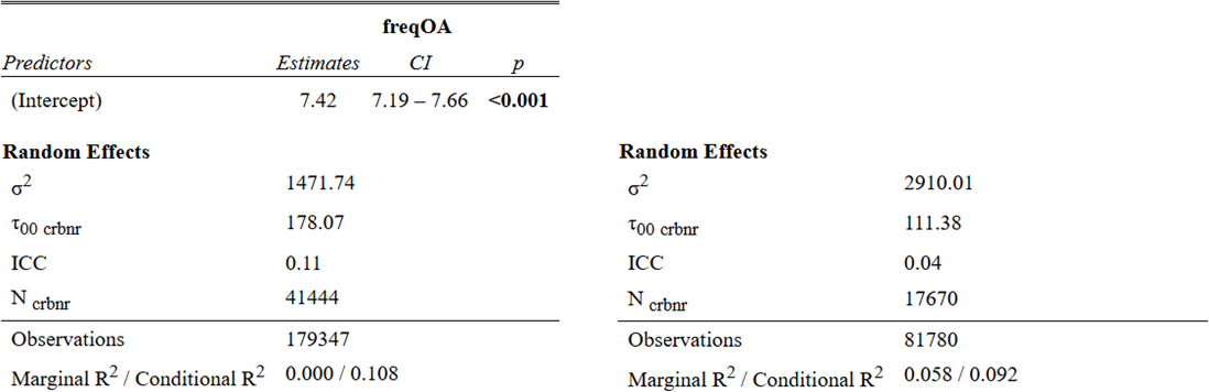
Significant determinants identified in the multivariable regression model, confirming the results of the corresponding univariable regression models, are ranked using the univariable regression model’s highest marginal/conditional R² ratios and reported with their multivariable regression estimates.
Determinants of the frequency degree include the following.
- Insurance companies. The estimates -5 lowest (\(\beta\) = -2.3), 9 highest (\(\beta\) = +15.6)- suggest that differences between OA insurers in some way are correlated with the mean frequency degrees of their clients. This represents a new finding that needs further investigation in future studies. See Section 1.3.4.4 and Section 3.4.3.5.
- Sector. Compared to agriculture, forestry an and fishing (level A), only construction (level F) and manufacturing (level C) show significant higher frequency degree estimates (\(\beta\) = +8.3 and \(\beta\) = +4.7, respectively). The lowest estimate is observed in accommodation and food service activities, (level I), with \(\beta\) = -10.2. The relative ranking of these results is in line with the frequency degrees reported in FEDRIS’ year report 2023 Fig 12.1c (Federal Agency for Occupational Risks, 2023). See Section 1.3.5 and Section 3.4.4.
- Company size. Compared to the smallest companies with <5 workers, all other size categories appear to be show higher frequency degrees, following a U-shaped relationship. The highest estimates are observed in category between 5-9 employees (\(\beta\) = +8.6) and in companies with >200 employees (\(\beta\) = +11.0). A more moderate increase of frequency degree is seen in the 20-49 employee companies (\(\beta\) = +4.5). See Section 1.3.4.2 and Section 3.4.3.2.
- Nature of the contract. A higher proportion of full-time workers significantly increases the frequency degree of a company (\(\beta\) = +4.7). See Section 1.3.3.3 and Section 3.4.2.3.
- Workforce segment. A higher proportion of blue-collar workers significantly increases the frequency degree of a company (\(\beta\) = +13.9). See Section 1.3.3.1 and Section 3.4.2.1.
- Salary level. Compared to having many workers in the highest earnings group (daily wage > € 250), having high proportions of workers in the segments <50 up to 125to149 workers significantly contributes to higher frequency degree estimates at company level (\(\beta\) = +6.9 to \(\beta\) = +8.5). See Section 1.3.2.5 and Section 3.4.1.5.
In practical terms, the model captures only a limited part of the observed variation in frequency degree, even after allowing every company being its own baseline via the random intercepts. This should not be interpreted as a failure of the modelling approach but rather aligns with expectations from the TRIR literature regarding short‑interval injury rates. Literature findings could be summarised as follows: OA are rare, subject to noise, and statistically unstable at the temporal resolution typically used in organisational reporting. While measures such as the frequency degree can provide directional insights and support risk stratification, they are not suitable for precise forecasting at the employer‑year level.
Variation in company-specific frequency degrees is highly random (>90%) and although factors such as insurer, sector, company size and other variables show statistical significance, their explanatory relevance remains limited
The multivariable model demonstrates limited explanatory power for frequency degrees. Occupational accident insurer companies, sector and size, and in employee fractions the nature of the contract, workforce segment and salary level have significant impacts on the model scores. However, if we consider the large portion unexplained variance (90.8%), the model is hardly useful in practice and confirms that caution is needed in using a TRIR-like safety measure such as the frequency degree at company level.
Figure 3.229 shows the different effect sizes of the categories included in the model. When compared with the previous model overviews, the figure shows wide confidence intervals indicating the high variability of frequency degrees.
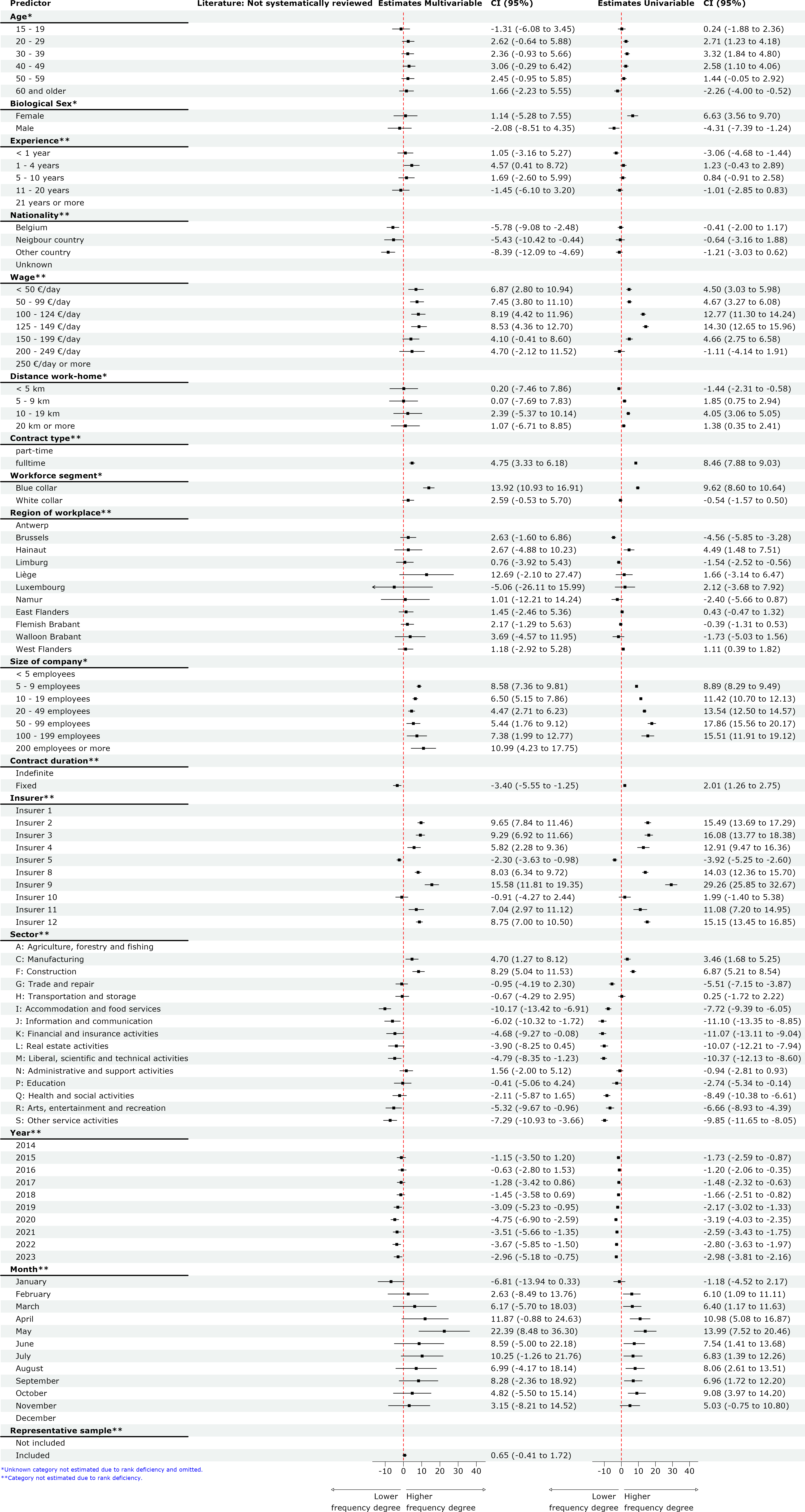
Potential biasses to be aware of when using TRIR-like metrics such as a frequency degree
- General underreporting. Our model’s nationality/region effects and negative coefficients for some groups might reflect reporting artifacts; peer reviewed studies document substantial undercounting and employer-level recordkeeping gaps (Azaroff et al., 2002; Rappin et al., 2016; Wuellner & Bonauto, 2014).
- Distorted reporting. When TRIR is used as a performance target -for example, in contracts or bonus schemes- it can unintentionally distort reporting behaviour. Borderline cases may go unrecorded, undermining TRIR’s reliability as a safety metric. This issue is particularly pronounced across jurisdictions with varying reporting standards and compensation incentives. In Belgium, this distortion is less likely to affect frequency rate reporting, as it falls under federal rather than regional legislation. However, the risk remains significant when TRIR- like measures are imposed as a performance targets for contractors or third parties. In such cases, the pressure to meet targets can lead to strategic underreporting, ultimately compromising the integrity of safety data.
- Confounding by workforce/industry mix, limiting cross-company benchmarking. Our large, significant effects for industry (e.g., Manufacturing “C”, Construction “F”), role mix (blue-collar, full-time) and establishment size mirror critiques that TRIR-like measures (such as a frequency degree) reflect many contextual factors beyond “safety performance” (Reiman & Pietikäinen, 2012)
- Sensitivty to tenure composition. Our positive/significant coefficient for the 1–4 year tenure band is consistent with elevated early-tenure injury risk (“new worker” risk), implying TRIR will swing with hiring/turnover independent of controls (Bena et al., 2013).
- Lagging indicators are of limited value for proactive control. The modest marginal R² and low ICC in our mixed model are consistent with the argument that lagging outcome metrics like TRIR capture multifactor results rather than system capability; leading/monitor indicators (e.g. safety training completion rates, near-miss reporting frequency, safety audits and inspections, PPE usage, safety engagement, hazard identification and risk reduction rate,…) are needed alongside measures as TRIR (Reiman & Pietikäinen, 2012).
3.5.7 Likelihood to experience a serious workplace OA (seriousOA, model 5)
This multilevel logistic multivariable regression model examines the factors associated with the likelihood an individual employed within a company experiences a serious workplace OA in a given month over the course of the ten-year study period (seriousOA).
The model includes 17,267 workplace OAs (0= no serious workplace OA, 1= serious workplace OA) for a given individual in a certain month, These observations span 14,198 unique individuals and 4,154 mutual ESPP/PS companies for which complete information on all model determinants is available.
Of the 17,267 workplace OAs, 1,136 are classified as serious, resulting in an overall individual chance of 6.6% for a workplace OA to be categorized as serious.
The random effect variance for individuals (insznr) is high (\(\tau_{00\,\text{insz}}\) = 552.81), indicating substantial unexplained heterogeneity at the individual level. Although the company-level variance is considerably lower (\(\tau_{00\,\text{crbnr}}\) = 4.14), suggesting that company affiliation does only contribute marginally to the classification of a workplace OA as serious, we retain the hierarchical clustering structure. This ensures accurate estimation of standard errors and facilitates meaningful comparison across models.
The model yields a conditional R² of 0.994, indicating that nearly all variation in classification the workplace OA as serious is explained when both fixed and random effects are considered. However, the marginal R² is only 0.005, showing that the fixed effects, such as part-time work, contribute virtually nothing in explaining this outcome. This suggests that the model’s explanatory power lies almost entirely in the between-individual variation, with the individual-level random effects accounting for nearly all of the explained variance. Properties and random effects of the full multivariable model (right) in comparison with the corresponding null model (left) are presented in Figure 3.230. Fixed effects estimates of the multivariable full model in comparison the corresponding univariable models and existing literature are shown in Figure 3.231.
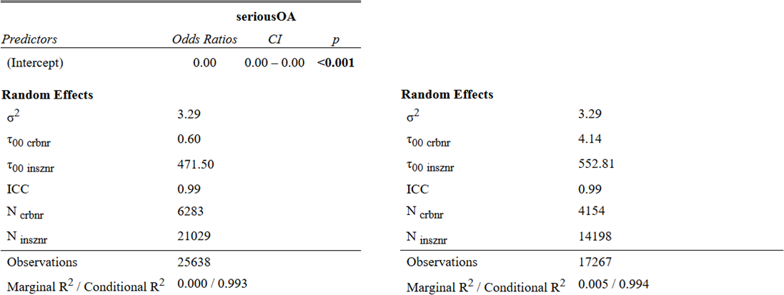
Significant determinants identified in the multivariable regression model, confirming the results of the corresponding univariable regression models, are ranked using the univariable regression model’s highest marginal/conditional R² ratios and reported with their multivariable regression OR.
Determinants of experiencing a serious OA include the following.
- Company size. Larger companies (200 workers and more) were associated with lower odds for serious workplace OA (OR = 0.13). See Section 1.3.4.2 and Section 3.4.3.2.
- Nature of the contract. Part-time workers had significantly lower odds for a serious workplace OA (OR = 0.38). See Section 1.3.3.3 and Section 3.4.2.3.
- Temporal factors. The odds of a serious workplace accident was significantly higher in 2020 (OR = 3.59) and 2023 (OR = 3.55), relatively to the reference year 2014. See Section 1.3.6 and Section 3.4.5.
The multivariable model identifies significant employer level (company size), individual level (nature of the contract) and temporal level (year) determinants that influence the classification of a workplace OA as serious. However, without adjustment for multiple testing, these results may be misleading and may represent false positives. Nevertheless, the finding that the largest employer segment (200 workers and more) is associated with lower odds for a serious accident is consistent with previous research (Kines & Mikkelsen, 2003), lending credibility to this specific result.
As for model 1.1 (statusOA, see Section 3.5.2), a similar caveat applies here. Since this model primarily includes demographic and employment-related variables (e.g. age, wage, nationality, company size), it lacks information on the specific circumstances of the accident itself (e.g. the different administrative codes that are used to classify a workplace OA as serious). As a result, its capacity to explain why a particular accident is classified as serious is inherently limited. This limitation reflects the scope of the model rather than a flaw, and underscores the importance of accident-specific variables in accurately capturing the severity of workplace accidents.
Size of the company and nature of the contract seems to be associated with classification of a workplace occupational accident as serious, but individual level variation and accident specific factors might be far more important
The model demonstrates strong fit at the individual level but weak explanatory power from fixed effects. The dominant source of variation is individual-level heterogeneity, with company affiliation playing only a minor role. The model’s utility for identifying systematic patterns for classifying a workplace occupational accident as serious is limited by the absence of accident-specific variables.
Figure 3.231 shows the different effect sizes of the categories included in the model. When compared with the model overview figures of the individual models 1, 2, and 3 (see Section 3.5.1, Section 3.5.3, and Section 3.5.4), the present figure displays wide confidence intervals, indicating high variability in the classification of a workplace OA as serious. We also observe that only a few of the whiskers (fewer than five) do not cross the reference line OR = 1.
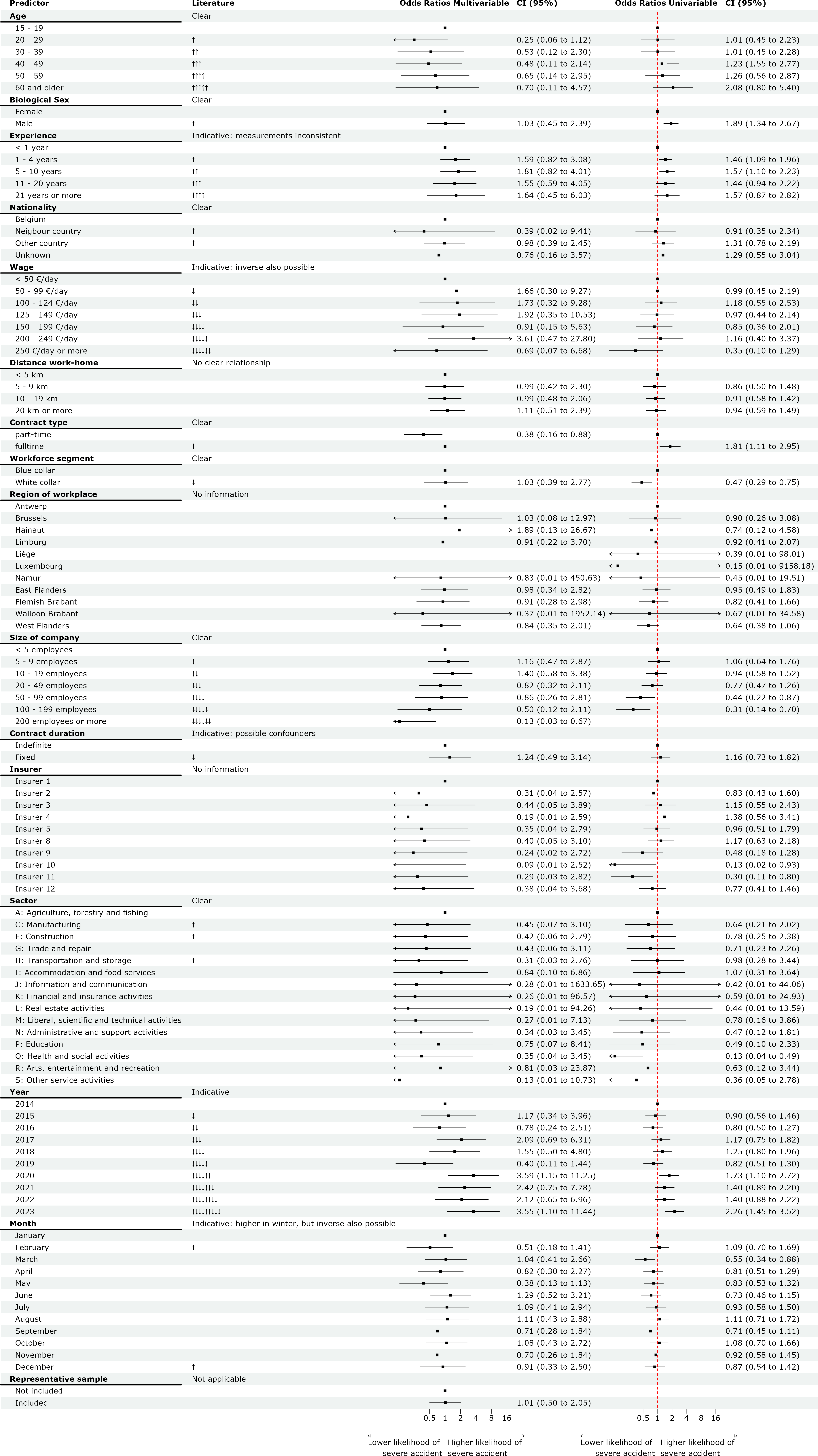
3.5.8 Days absent (validated) due to a workplace OA (nDaysTAO, model 6)
This multilevel multivariable regression model examines the factors associated with the IRR of the number of days absent due to a workplace OA over the ten-year study period (nDaysTAO).
The model includes 17,287 workplace OA across 4,168 mutual ESPP/PS companies for which complete information on all model determinants is available.
In the dataset used for this model, a substantial number of workplace OA (5,867 cases or 33.9%) result in zero days of absence from work. The median duration of absence is 5 days, while the mean is 24 days absence.
The model includes both fixed effects (company-level predictors) and random effects (group-level variation across companies over time). With a marginal R² of 0.200 and a conditional R² of 0.330, the model explains a substantial portion of the variance. This indicates that group-level factors substantially contribute to the outcome. The ICC was 0.16, suggesting that only 16% of the variance is attributable to differences between companies. Since the ICC is larger than 0.10, the use of a multilevel approach is justified (Section 3.2.2.2).
The model yields a relatively high R² ratio (0.61), indicating that most of the explained variance is attributable to fixed effects. Since the total explained variance is also relatively good, the identified fixed effects can be considered as valuable determinants. Properties and random effects of the full multivariable model (right) in comparison with the corresponding null model (left) are presented in Figure 3.232. Fixed effects estimates of the multivariable full model in comparison the corresponding univariable models and existing literature are shown in Figure 3.233.
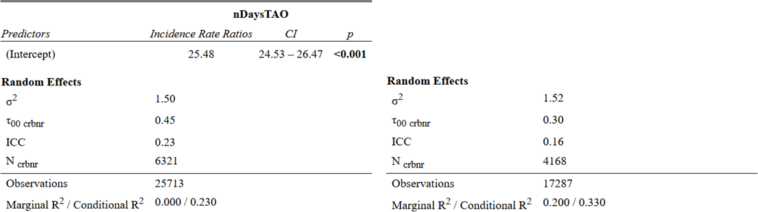
Significant determinants identified in the multivariable regression model, confirming the results of the corresponding univariable regression models, are ranked using the univariable regression model’s highest marginal/conditional R² ratios and reported with their multivariable regression IRR.
Determinants of the FEDRIS-validated number of days absent due to a workplace OA include the following.
- Age. The IRR gradually increases from 1.49 for workers in their twenties, to 5.30 for those aged 60 and above. This pattern confirms the commonly observed trend that older workers tend to have longer duration of work absence. See Section 1.3.3.3 and Section 3.4.2.3.
- Sector. Compared to agriculture, forestry and fishing sector (level A), the lowest incidence rate ratios for days absent can be found in sectors M (Professional, scientific and technical activities, IRR = 0.41), L (Real estate activities, IRR = 0.49) and S (Other Service activities). The highest IRR was found in sector F (construction, IRR = 1.16) although this difference was not statistically significant compared to level A. See Section 1.3.5 and Section 3.4.4.
- Company size. Compared to the reference category of companies with <5 than employees, the IRR for the number of days absent gradually decreases as company size increases, ranging from an IRR of 0.85 in the 20-49 employee segment to 0.72 in companies with 200 or more employees. This confirms previous literature indicating that smaller companies report more lost workdays following a workplace OA (Kines & Mikkelsen, 2003). See Section 1.3.4.2 and Section 3.4.3.2.
- Workforce segment. Employees with a white-collar status showed a substantially lower IRR (IRR = 0.85) for the validated number of days absent. See Section 1.3.3.1 and Section 3.4.2.1.
- Work experience. Longer work experience was associated with higher IRR for the validated number of days absent, with an increasing trend from 1.14 for employees with 1–4 years of experience to 1.31 for those with \(\geq\) 21 years (IRR = 1.31). See Section 1.3.2.3 and Section 3.4.1.3.
- Insurance companies. IRR varied notably between OA insurers, ranging from 0.61 (Insurer 11) to 1.17 (Insurer 9). This suggests that differences between OA insurers in some way affect the number of days absent. This is a new finding that needs confirmation in future studies. See Section 1.3.4.4 and Section 3.4.3.5.
- Salary level. Wage categories were associated with IRR of the number of days absent due to a workplace OA. Compared to the reference category of less than €50 daily wage, the highest IRR was observed in the €50–99 bracket (IRR = 1.31), while the lowest was found in the highest wage category of \(\geq\) €250 (IRR = 0.64). See Section 1.3.2.5 and Section 3.4.1.5.
- Nature of the contract. Part-time workers had significantly lower IRR for validated days of absence (IRR = 0.75). See Section 1.3.3.3 and Section 3.4.2.3.
- Temporal effects. The IRR for the number of days absent due to a workplace OA was significantly higher in 2016, 2019, 2021 and 2022, compared to 2014. Additionally, accidents occurring in July were associated with significantly lower IRR (IRR = 0.85) compared to those occurring in January. See Section 1.3.6 and Section 3.4.5.
The multivariable model highlights that individual-level factors (age, work experience, workforce segment, salary level, nature of the contract), employer-level factors conditions (sector, insurer, size), and temporal factors (year and month) are significant determinants of the validated number of days absent.
Although specific parameters of the OA itself (not included in the current model) may have a substantial impact on the number of days absent (Federal Public Service Health, Food Chain Safety and Environment, 2022), present findings indicate that general group-level predictions can be made. The determinants from the current model allow for the estimation of absence profiles at the company-level due to workplace OA.
Age, sector and size of the company are valuable determinants to estimate a number of (FEDRIS-validated) days absent from work, even without any specific information of the occupational accident itself
The multivariable model demonstrates high explanatory power for the (FEDRIS validated) number of days absent from work following a workplace occupational accident. Age, sector and company size have the highest marginal to conditional R² proportions in their corresponding univariable models. Company-level heterogeneity plays an important role and has to be taken into account.
Figure 3.233 shows the different effect sizes of the categories included in the model. The figure immediately indicates large effects for e.g. age and sector since their estimates (dots with whiskers) lie relatively further from the IRR = 1 reference line compared to the other variables included in the model.
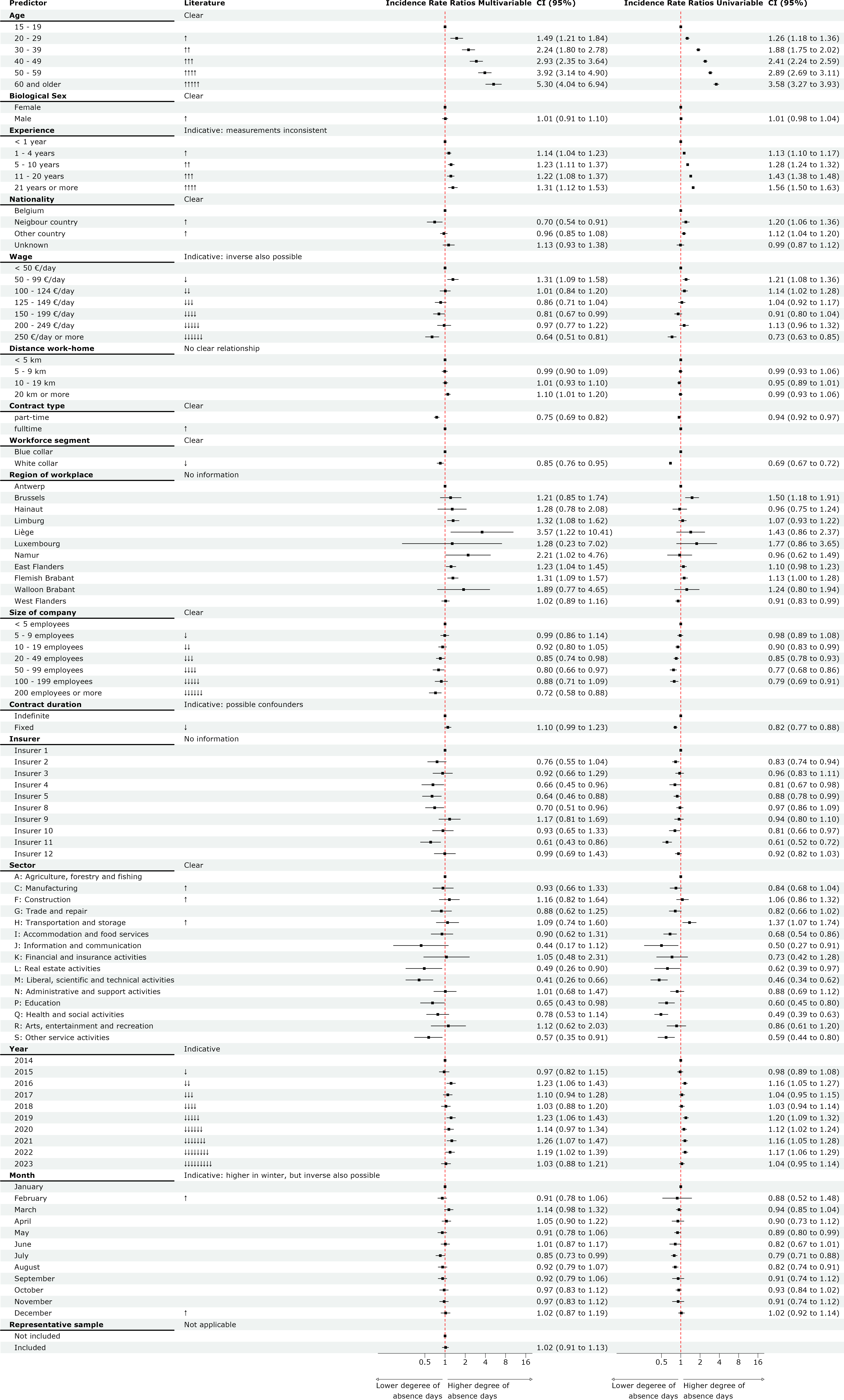
3.5.9 Days absent (calculated) due to a workplace OA (lengtecor, model 6.1)
This multilevel multivariable regression model is completely analogous to the previous model. It examines the factors associated with the IRR of the number of days absent due to a workplace OA over the ten-year study period, but this time using absence duration calculated by Liantis (lengtecor).
This measure is derived directly from Liantis PS calendars, allowing for immediate estimation of absence duration without waiting for external validation by a governmental instance (i.e. FEDRIS, which kindly provided the validated absence data used in the previous model, see Section 2.6).
The model includes 9,822 workplace OA across 2,946 mutual ESPP/PS companies, for which complete information on all included determinants is available.
A notable proportion of cases (477, or 4.9%) in the dataset used for this model result in zero days of absence from work. The median calculated absence duration following a workplace OA is 10, and the mean is 33 days.
The model incorporates both fixed effects (company-level predictors) and random effects (group-level variation across companies over time). With a marginal R² of 0.111 and a conditional R² of 0.381, the model explains a moderate portion of the variance, indicating that group-level factors contribute substantially to the outcome. The ICC of 0.30, suggests that 30% of the variance is attributable to differences between companies. Since the ICC is much larger than 0.10, the use of a multilevel approach is justified (Section 3.2.2.2).
The relatively high conditional R² compared to the marginal R² (ratio of 0.29) indicates that company-level heterogeneity plays an important role. The fixed effects identified in the model can therefore be considered valuable determinants of calculated absence duration. Properties and random effects of the full multivariable model (right) in comparison with the corresponding null model (left) are presented in Figure 3.234. Fixed effects estimates of the multivariable full model in comparison the corresponding univariable models and existing literature are shown in Figure 3.235.
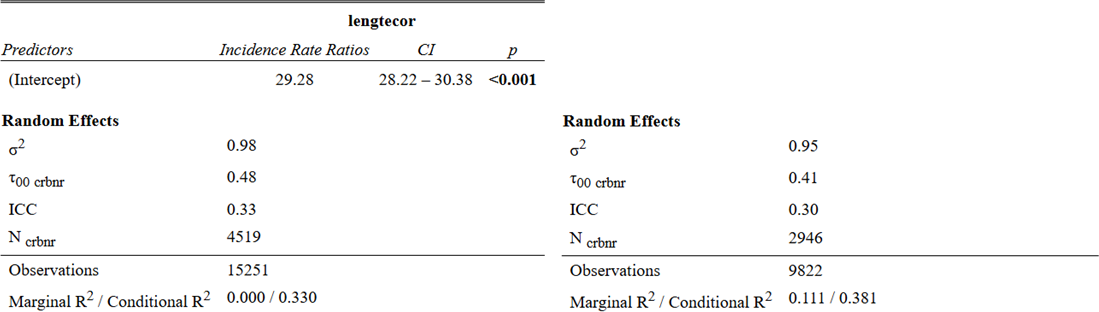
Significant determinants identified in the multivariable regression model, confirming the results of the corresponding univariable regression models, are ranked using the univariable regression model’s highest marginal/conditional R² ratios and reported with their multivariable regression IRR.
Determinants of the (Liantis-calculated) number of days absent due to a workplace OA include the following.
- Age. The IRR progressively increases from 1.64 for workers in their twenties, to 3.93 for those aged 60 or more. This confirms the trend that older workers tend to be absent longer following an OA. See Section 1.3.3.3 and Section 3.4.2.3.
- Sector. Compared to agriculture, forestry and fishing (level A), the lowest IRR values were found in sectors M (Professional, scientific and technical activities, IRR = 0.41) and L (Real estate activities, IRR = 0.41), while sector F (Construction) did not show a significant difference (IRR = 0.97, ns). See Section 1.3.5 and Section 3.4.4.
- Work experience. Longer work experience was associated with higher IRR, with a clear increasing trend from 1–4 years (IRR = 1.13) to \(\geq\) 21 years (IRR = 1.43). See Section 1.3.2.3 and Section 3.4.1.3.
- Company size. Compared to companies with <5 employees, the number of days absent decreases as company size increases. Significant reductions were observed in the 20–49 segment (IRR = 0.80), 50–99 (IRR = 0.75), and \(\geq\) 200 (IRR = 0.80). These findings support earlier research that smaller companies tend to report more lost workdays following an OA (Kines & Mikkelsen, 2003). However, the overall trend appears somewhat less clear than in the previous model. See Section 1.3.4.2 and Section 3.4.3.2.
- Workforce segment. White-collar employees had significantly higher IRR (IRR = 1.17), which contrasts with the validated model where they had lower IRR. This difference should be further investigated. See Section 1.3.3.1 and Section 3.4.2.1.
- Insurance companies. The variation observed between insurers, ranging from IRR = 0.77 (lowest, insurers 11 and 5) to IRR = 1.14 (highest, insurer 9), is consistent with the direction and magnitude in the former model. However, in the current model, this difference does not reach statistical significance. See Section 1.3.4.4 and Section 3.4.3.5.
- Temporal effects. As in the previous model based on the validated absence data, the years 2019, 2021, and 2022 show the highest estimates for absence duration. However, this difference is not statistically significant compared to the reference year 2014. While the previous model identified July as the month with a notably lower IRR, the current model highlights August as significantly lower (IRR = 0.85). Together, both models suggest possible seasonal (summer) and/or holiday-related effects influencing absence duration. See Section 1.3.6 and Section 3.4.5.
The current multivariable model demonstrates that individual-level factors (age, work experience, workforce segment), employer-level conditions (sector, company size), and temporal factors (month) are significant determinants of the Liantis-calculated number of days absent. Although OA-specific parameters (e.g. injury type, severity) are not included, the model allows for group-level predictions of absence profiles based on structural characteristics.
Age, sector, and company size again emerge as strong predictors, confirming their utility in estimating group_level absence duration without needing OA specific information post occurrence of the accident. The model’s explanatory power, especially the high conditional R², underscores the importance of accounting for company-level heterogeneity in absence modeling.
Age, sector and size of the company are valuable determinants to estimate a number of (Liantis-calculated) days absent from work, even without any specific information of the occupational accident itself
The multivariable model demonstrates high explanatory power for the Liantis-calculated number of days absent from work following a workplace occupational accident. Age, sector and company size have the highest marginal to conditional R² proportions in their corresponding univariable models. Company-level heterogeneity plays an important role and has to be taken into account.
Figure 3.235 shows the different effect sizes of the categories included in the model. The figure immediately indicates large effects for e.g. age and sector since their estimates (dots with whiskers) lie relatively further from the IRR=1 reference line compared to the other variables included in the model.
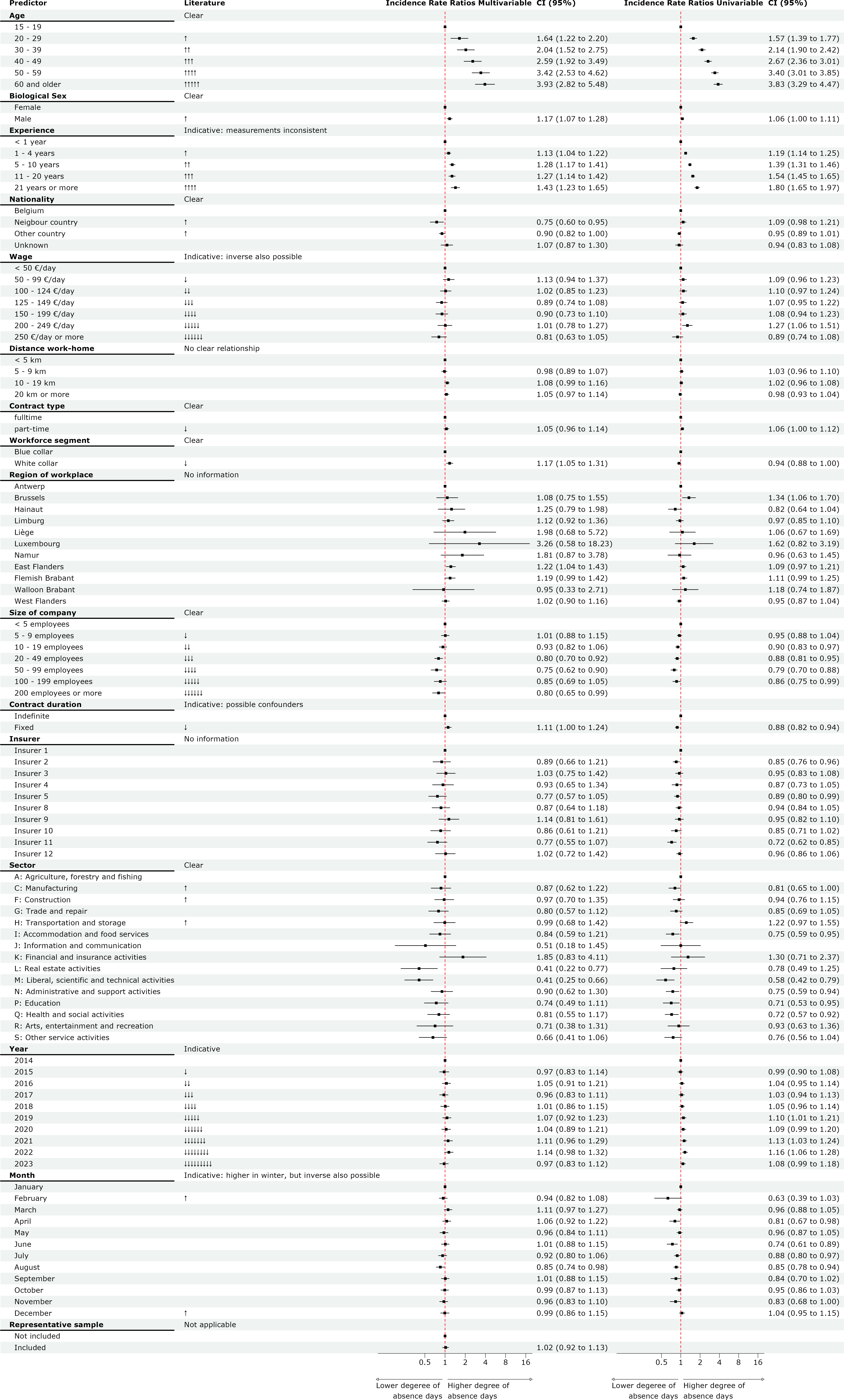
3.5.10 Days absent modelling results compared
Liantis’ internally calculated number of days absent following a workplace OA -used in model 6.1 (Section 3.5.9)- appears to be a valid and useful proxy for modelling absence duration. However, this variable (lengtecor) is not a perfect substitute for the validated government variable (nDaysTAO) used in model 6 (Section 3.5.8).
Model 6.1 relies on Liantis’ internal data, which is more readily accessible and can be processed quickly. This makes it particularly valuable when validated data are not (yet) available. Although FEDRIS provided validated data for this study, there is currently no formal mechanism to access such data on a case-by-case basis outside this research context. As a result, the operational usefulness of model 6 remains limited.
Model 6, which uses validated absence data, explains more variance in absence duration (marginal R² = 0.200 vs 0.111), suggesting that it is more precise and captures a broader range of real-world variation. Additionally, the number of observations is nearly double (17,287 validated vs 9,822 calculated), reinforcing our earlier recommendation: it would be highly beneficial to structurally share the “final truth” concerning the number of days absent following an OA alongside the definitive status of closed OA files.
Only half of the validated cases could be processed directly via Liantis
Further research is needed to refine the algorithm that estimates absence duration using Liantis PS calendars since absence could only be estimated for 9,822 of the 17,287 validated cases.
Structurally sharing key outcomes with stakeholders would increase value for all parties
Critical outcomes -such as the final number of days absent, total cost of the accident, final dossier status, and seriousness of the OA- are currently not shared across stakeholders in a structured way. This limits the potential for evidence-based prevention and hinders efforts to support reintegration and return-to-work strategies.
Some predictors (such as age) exhibit stronger effects in the model based on validated data (Model 6), suggesting that this model captures more nuanced or extreme cases. In contrast, Model 6.1 tends to attenuate these effects, likely due to estimation errors or missing details in the internal algorithm used to calculate absence duration. Interestingly, Model 6.1 identifies a significant effect for biological sex, with men appearing to have significantly more calculated absence days. However, since this effect is not observed in Model 6, further research is needed to determine whether this finding reflects a true underlying difference or is merely an artifact of the internal calculation method. Interestingly, the higher ICC in model 6.1 (0.30 vs 0.16 in model 6) suggests stronger clustering by employer or sector. This may reflect systematic biases or limitations in how internal absence data is structured or recorded.
Use model 6.1 for operational monitoring and early warning; model 6 for research and validation
Given the easier accessibility of the source data and the reasonable predictive power, model 6.1 might be suited for operational use and early warning systems. If validated data were to become structurally available, hybrid models combining internal and external sources could be developed to enhance accuracy without sacrificing timeliness. Continued validation of both models is recommended, along with further investigation into discrepancies to identify potential biases and improve the internal absence calculation algorithm.
3.5.11 Direct wage cost due to a workplaceOA (costOA, model 7)
This multilevel multivariable regression model explores the determinants of the log-transformed cost (base 10) of OA over the ten-year study period. To avoid results approaching minus infinity, one euro was added to the cost variable, resulting in the transformation: \(\log_{10}(\text{costOA} + \text{€}1)\). This transformation was applied to reduce skewness and stabilize variance in the cost distribution.
The model includes 20,423 observations across 4,105 mutual ESPP/PS companies for which complete information on all included determinants is available.
In the dataset used for this model, a substantial proportion of workplace OA (5,370 cases, or 26.3%) result in €0 direct wage cost. The median cost is €867 (corresponding to 2.94 on the log scale), while the mean cost, reflecting a highly skewed distribution, was €180.
The model includes both fixed effects (company-level predictors) and random effects (group-level variation across companies in time). With a marginal R² of 0.153 and a conditional R² of 0.378, it explains a substantial portion of the variance in OA-related costs. This indicates that group-level factors (differences between companies) contribute substantially to the outcome. The ICC of 0.27 suggests that 27% of the variance is attributable to differences between companies. Given that the ICC exceeds the commonly accepted threshold of 0.10, the use of a multilevel approach is justified (Section 3.2.2.2).
The R² ratio is relatively high (0.40), meaning that a moderate share of the explained variance in cost comes from fixed effects. Given the total explained variance is also relatively good, these fixed effects can be considered as valuable determinants of the direct wage cost due to a workplace OA. Properties and random effects of the full multivariable model (right) in comparison with the corresponding null model (left) are presented in Figure 3.236. Fixed effects estimates of the multivariable full model in comparison the corresponding univariable models and existing literature are shown in Figure 3.237.
Significant determinants identified in the multivariable regression model, confirming the results of the corresponding univariable regression models, are ranked using the univariable regression model’s highest marginal/conditional R² ratios and reported with their multivariable regression estimates.
Determinants of the (log-transformed) cost of workplace OAs include the following.
- Workforce segment. White-collar workers show significantly lower costs (\(\beta\) = -0.30). See Section 1.3.2.2 and Section 3.4.1.2.
- Sector. Several sectors are significantly associated with cost differences. For example, transport (level H, \(\beta\) = 0.45) and construction (level F, \(\beta\) = 0.39) show higher costs, while education (level P, \(\beta\) = -0.39) and information & communication (level J, \(\beta\) = -0.58) are associated with lower costs. These findings are consistent with previously described sector-specific risk profiles. For example, in the transport sector, road traffic accidents are often classified as workplace (rather than commuting) OAs and such accidents on the road tend to result in more severe consequences. See Section 1.3.5 and Section 3.4.4.
- Nature of the contract. Part-time employment is associated with lower costs (\(\beta\) = -0.08), which may reflect differences in exposure duration or job type . See Section 1.3.3.3 and Section 3.4.2.3.
- Age. Compared to the reference group (<20 years), direct wage costs increase with age. The effect becomes statistically significant from the 40–49 age group (\(\beta\) = 0.22) and remains so in older groups (e.g., 60+: \(\beta\) = 0.29). This aligns with previous findings that older workers tend to experience more severe injuries when workplace OA occur (although they show lower likelihoods to experience such workplace OA). Our study thus confirms both patterns described in the literature. See Section 1.3.2.1 and Section 3.4.1.1.
- Salary level. A positive but diminishing gradient is observed: for instance, workers earning €50–99/day show an estimate of \(\beta\) = 1.72 in comparison with the lowest category.Lower but still substantial effects can be noticed in higher brackets e.g. \(\beta\) = 1.32 for workers earning \(\geq\) €250. See Section 1.3.2.5 and Section 3.4.1.5.
- Company size. Employees in medium-sized firms (brackets 50-99, \(\beta\) = 0.22, to 200–499 employees, \(\beta\) = 0.29) tend to generate slightly higher direct wage costs, possibly due to more formalized reporting procedures or higher average wages. See Section 1.3.4.2 and Section 3.4.3.2.
- Work experience. Longer work experience was associated with higher direct costs, with an increasing trend from 1–4 years (\(\beta\) = 0.09) to \(\geq\) 21 years (\(\beta\) = 0.18). See Section 1.3.2.3 and Section 3.4.1.3.
- Insurance companies. Some significant effects can be noticed, e.g. insurer 9 (\(\beta\) = 0.66), 11 (\(\beta\) = 0.34) and 12 (\(\beta\) = 0.28) are associated with higher direct wage costs. This is a new finding that needs confirmation in future studies. See Section 1.3.4.4 and Section 3.4.3.5.
- Temporal effects. In comparison to 2014, a kind of upward trend can be observed. Direct wage costs increase notably from 2016 onwards, with the highest costs occurring in 2021 (\(\beta\) = 0.30). Seasonal variation is also apparent: with May (\(\beta\) = -0.08) and December (\(\beta\) = -0.10) showing lower cost estimates compared to January. See Section 1.3.6 and Section 3.4.5.
The multivariable model highlights that individual-level factors (age, work experience, workforce segment, salary level, nature of the contract), employer-level factors (sector, size, insurer), and temporal factors (year and month) are significant determinants of the direct wage cost resulting from a workplace OA.
This means that, although the specific accident-related parameters (not included in the model) might have a very significant and relevant effect on the cost, also group-level estimates can be made using the determinants from the current model to predict group-level cost profiles due to workplace OA.
Sector, size, workforce, age and wage are valuable determinants to estimate the direct wage costs due to workplace occupational accident
The multivariable model demonstrates good explanatory power for the Liantis registered direct wage costs following workplace occupational accidents. Among the determinants, company-level factors, such as sector and company size, and individual-level determinants, such as workforce, age and wage have the highest marginal to conditional R² proportions in their corresponding univariable models. These findings highlight the importance of company-level heterogeneity, which must be accounted for in cost estimations.
Figure 3.237 shows the different effect sizes of the categories included in the model. The figure immediately indicates large effects for e.g. wage and sector since their estimates (dots with whiskers) lie relatively further from the grand mean = 0 difference reference line compared to the other variables included in the model.
3.5.12 Severity degree (validated absence) of workplace OA (sevOAval, model 8)
This multilevel multivariable regression model investigates the factors associated with the severity degree of a company in a given year over the ten-year study period (sevOAval).
The model includes 82,989 annual observations (representing the severity degree for a given company in a given year), across 17,735 unique mutual ESPP/PS companies for which complete information on all determinants included in the model is available.
Many companies do not experience workplace accidents that have to be included in the calculation of the severity degree. As a result, both the median and 75ile of severity degree are zero. The overall mean severity degree across all companies, being strongly influenced by the larger values of companies with such countable OAs, is 1.1.
The model includes both fixed effects (company-level predictors) and random effects (group-level variation across companies in time). However, with a marginal R² of 0.010 and a conditional R² of 0.016, it explains only a very small fraction of the variance, leaving 98.4% unexplained. This indicates that group-level factors do not substantially contribute to the outcome. The ICC was 0.01, suggesting that only 1% of the variance is attributable to differences between companies and that most variance is within companies over time rather than between companies. Although an ICC smaller than 0.10 implies that a multilevel approach is not strictly necessary, its use facilitates comparison with other models (Section 3.2.2.2).
The R² ratio is relatively high (0.010 / 0.016 = 0.63), indicating that most of the explained variance comes from fixed effects. However, given the total explained variance is very low, these fixed effects cannot be considered strong determinants of the outcome. Properties and random effects of the full multivariable model (right) in comparison with the corresponding null model (left) are presented in Figure 3.238. Fixed effects estimates of the multivariable full model in comparison the corresponding univariable models and existing literature are shown in Figure 3.239.
Significant determinants identified in the multivariable regression model, confirming the results of the corresponding univariable regression models, are ranked using the univariable regression model’s highest marginal/conditional R² ratios and reported with their multivariable regression estimates.
Determinants of the severity degree (validated absence) include the following.
- Sector. Compared to agriculture, forestry and fishing (A), significantly lower severity degrees are observed in level I (accommodation & food service activities, \(\beta\) = -1.15) and level S (other service activities, \(\beta\) = -0.99). No statistically significant differences are found between level A and the remaining sectors. See Section 1.3.5 and Section 3.4.4.
- Insurance companies. Relative to the reference insurer, several insurers are associated with higher average severity degrees such as insurer 9 (\(\beta\) = +1.03) and insurer 3 (\(\beta\) = +0.86). In contrast, insurer 5 shows a lower average severity degree (\(\beta\) = -0.28). These findings suggest that differences between OA insurers correlate with the mean employer-year severity degrees. This this is a novel finding that warrants confirmation in future studies. See Section 1.3.4.4 and Section 3.4.3.5.
- Workforce segment. A higher fraction of bluecollar workers (arbeiders) is associated with a higher severity degree (\(\beta\) = +3.76). See Section 1.3.3.1 and Section 3.4.2.1.
- Salary level. A higher fraction of low-wage workers (day wage <50) is significantly associated with a higher severity degree (\(\beta\) = +2.59). In contrast, mid-range and high-wage salary fractions do not significantly seem to contribute. See Section 1.3.2.5 and Section 3.4.1.5.
- Company size. Compared to the smallest companies (<5 workers), significantly lower severity degrees are observed in larger company ize categories: 5–9 employees (\(\beta\) = -0.51), 10–19 employees (\(\beta\) = -0.71), 20–49 employees (\(\beta\) = -0.80) and 50–99 employees (\(\beta\) = -0.79). See Section 1.3.4.2 and Section 3.4.3.2.
- Age. Only fractions in ages groups 40–49 years (\(\beta\) = +0.80) and 50–59 years(\(\beta\) = +1.16) seem to be associated with higher severity degrees. See Section 1.3.2.1 and Section 3.4.1.1.
- Temporal factors. Severity degrees are significantly lower in 2020 (\(\beta\) = -0.84), 2021 (\(\beta\) = -0.60), 2022 (\(\beta\) = -0.55) and 2023 (\(\beta\) = -0.90) relative to the reference year. This pattern is consistent with a downward shift during and following the COVID-19 pandemic. See Section 1.3.6 and Section 3.4.5.
In practical terms, the model captures only a very small part of the observed variation in severity degrees, even after accounting for company-specific baselines through the inclusion of random intercepts. Similar remarks apply as the ones noted for the frequency degree model. Therefore, we do not recommend using severity degrees as point-precise measures at the employer-year level.
The variation in company-specific severity degrees appears largely random, with over 98% of the variance remaining unexplained. Although sector, insurer, workforce segment, salary level, company size, age and time (years) show statistically significant associations with the severity degree, their explanatory power is modest relative to the overall variability, limiting their practical utility as predictive factors.
The multivariable model demonstrates low explanatory power for severity degrees. Occupational accident insurer, sector and size, and in employee fractions the workforce segment, salary level and parts of the age distribution have significant impacts on the model scores. However, the model is hardly useful in practice and confirms that caution is needed when using such a measure for benchmarking at company level.
Variation in company-specific severity degrees (validated absence) is highly random (>98%) and although factors such as insurer, sector, company size and other variables show statistical significance, their explanatory relevance remains limited
The multivariable model demonstrates only very limited explanatory power for severity degrees. Occupational accident company insurers, sector and size, and in employee fractions the workforce segment, salary level and age have significant impacts on the model scores. However, if we consider the large portion unexplained variance (98.4%), the model is hardly useful in practice and confirms that caution is needed in using this safety measure at the company level.
Figure 3.239 shows the different effect sizes of the categories included in the model. When compared with Figure 3.221, Figure 3.225 and Figure 3.227, the figure shows wide confidence intervals indicating the high variability of severity degrees.
3.5.13 Severity degree (calculated absence) of workplace OA (sevOAcal, model 8.1)
In this final multilevel multivariable regression model, we examine the factors associated with severity degree of a company in a given year over the ten-year study period (sevOAcal). Unlike the previous model, this analysis uses Liantis-calculated absence days and not the FEDRIS validated absence days.
The model includes 83,000 yearly observations (representing the severity degree for a given company in a given year), across 17,740 unique mutual ESPP/PS companies for which complete information on all determinants included in the model is available.
As in the previous model, many companies do not experience workplace OA that contribute to the calculation of the severity degree. Consequently, both the median and 75th percentile severity degree are zero. The overall mean severity degree across all companies remains approximately 0.9, largely driven by the higher values observed in companies with such countable OAs.
The model includes both fixed effects (company-level predictors) and random effects (group-level variation across companies in time). However, with a marginal R² of 0.007 and a conditional R² of 0.016, the model explains only a very small fraction of the variance, leaving 98.4% unexplained. The ICC is 0.01, indicating that only 1% of the variance is attributable to differences between companies, and most variance occurs within companies over time rather than between companies. As in the previous model, the use of a multilevel approach is not strictly required but facilitates comparison with other models (Section 3.2.2.2).
The ratio of marginal to conditional R² (0.007 / 0.016 = 0.44) suggests that most of the explained variance still comes from fixed effects, but since total explained variance is very low, these fixed effects cannot be considered strong determinants. Properties and random effects of the full multivariable model (right) in comparison with the corresponding null model (left) are presented in Figure 3.240. Fixed effects estimates of the multivariable full model in comparison the corresponding univariable models and existing literature are shown in Figure 3.241.
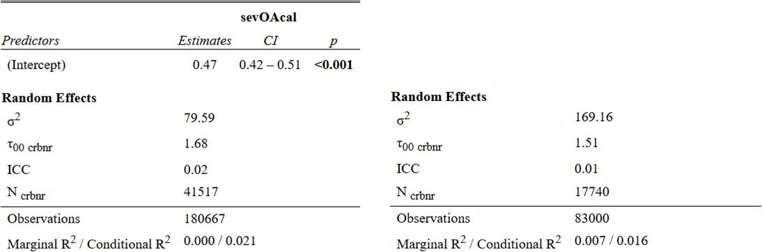
Significant determinants identified in the multivariable regression model, confirming the results of the corresponding univariable regression models, are ranked using the univariable regression model’s highest marginal/conditional R² ratios and reported with their multivariable regression estimates.
Determinants of the severity degree (calculated absence) include the following.
- Sector. Compared to agriculture, forestry and fishing (level A), significantly lower severity degrees are observed in several sectors, including level I (accommodation & food service activities, \(\beta\) = -1.39), level S (other service activities, \(\beta\) = -1.35), and others such as the levels G, J, K, L, M, P, Q, R (all negative and significant). This pattern is more pronounced than in the previous model Section 3.5.12. See Section 1.3.5 and Section 3.4.4.
- Insurance companies. Compared to the reference insurer, some insurers are associated with higher average severity degrees, such as insurer 9 (\(\beta\) = +1.21) and insurer 3 (\(\beta\) = +0.92), while others show either lower or non-significant effects. This is a novel finding that warrants confirmation in future studies. See Section 1.3.4.4 and Section 3.4.3.5.
- Workforce segment. A higher fraction of blue-collar workers (arbeiders) is associated with higher severity degree (\(\beta\) = +3.71). See Section 1.3.3.1 and Section 3.4.2.1.
- Salary level. A higher fraction of low daily wage earners (day wage <50) is associated with increased severity degree (\(\beta\) = +3.22). The effect is even larger than in the previous model. In contrast, midrange and high salary fractions do not significantly contribute. See Section 1.3.2.5 and Section 3.4.1.5.
- Company size. Relative to the smallest companies (<5 workers), the severity degree is lower in company size classes with 5–9 (\(\beta\) = -0.58), 10–19 (\(\beta\) = -0.74), 20–49 (\(\beta\) = -0.82), and 50–99 employees (\(\beta\) = -0.85). See Section 1.3.4.2 and Section 3.4.3.2.
- Age. Only the fraction of workers in age category 50–59 years shows a significant positive association (\(\beta\) = +0.79) with the severity degree. See Section 1.3.2.1 and Section 3.4.1.1.
- Temporal factors. The severity degrees are significantly lower in the years 2018 (\(\beta\) = -0.58), 2020 (\(\beta\) = -0.90), 2021 (\(\beta\) = -0.74), 2022 (\(\beta\) = -0.65), and 2023 (\(\beta\) = -0.81) compared to the reference year, reflecting a downward trend during and following the COVID-19 period. See Section 1.3.6 and Section 3.4.5.
In practical terms, the model captures only a very small part of the observed variation in severity degrees, even after accounting for company-specific baselines through the inclusion of random intercepts. Similar remarks apply as the ones noted for the frequency degree model. Therefore, we do not recommend using severity degrees as point-precise measures at the employer-year level.
The variation in company-specific severity degrees appears largely random, with over 98% of the variance remaining unexplained. Although sector, insurer, workforce segment, salary level, company size, age and time (years) show statistically significant associations with the severity degree, their explanatory power is minimal relative to the overall variability, limiting their practical utility as predictive factors.
The multivariable model demonstrates low explanatory power for severity degrees. Although variables such as OA insurer, sector and company size, and employee-fractions of the workforce segment, salary level, and certain age group fractions have significant impact on the severity degree, the model is hardly useful in practice. These findings confirms that caution is needed when employing such measures for benchmarking at the company level.
Variation in company-specific severity degrees (calculated absence) is highly random (>98%) and although factors such as insurer, sector, company size and other variables show statistical significance, their explanatory relevance remains limited
The multivariable model demonstrates only very limited explanatory power for severity degrees. Occupational accident company insurers, sector and size, and in employee fractions the workforce segment, salary level and age have significant impacts on the model scores. However, if we consider the large portion unexplained variance (98.4%), the model is hardly useful in practice and confirms that caution is needed in using this safety measure at the company level.
Figure 3.241 shows the different effect sizes of the categories included in the model. When compared with Figure 3.221, Figure 3.225 and Figure 3.227, the figure shows wide confidence intervals indicating the high variability of severity degrees.
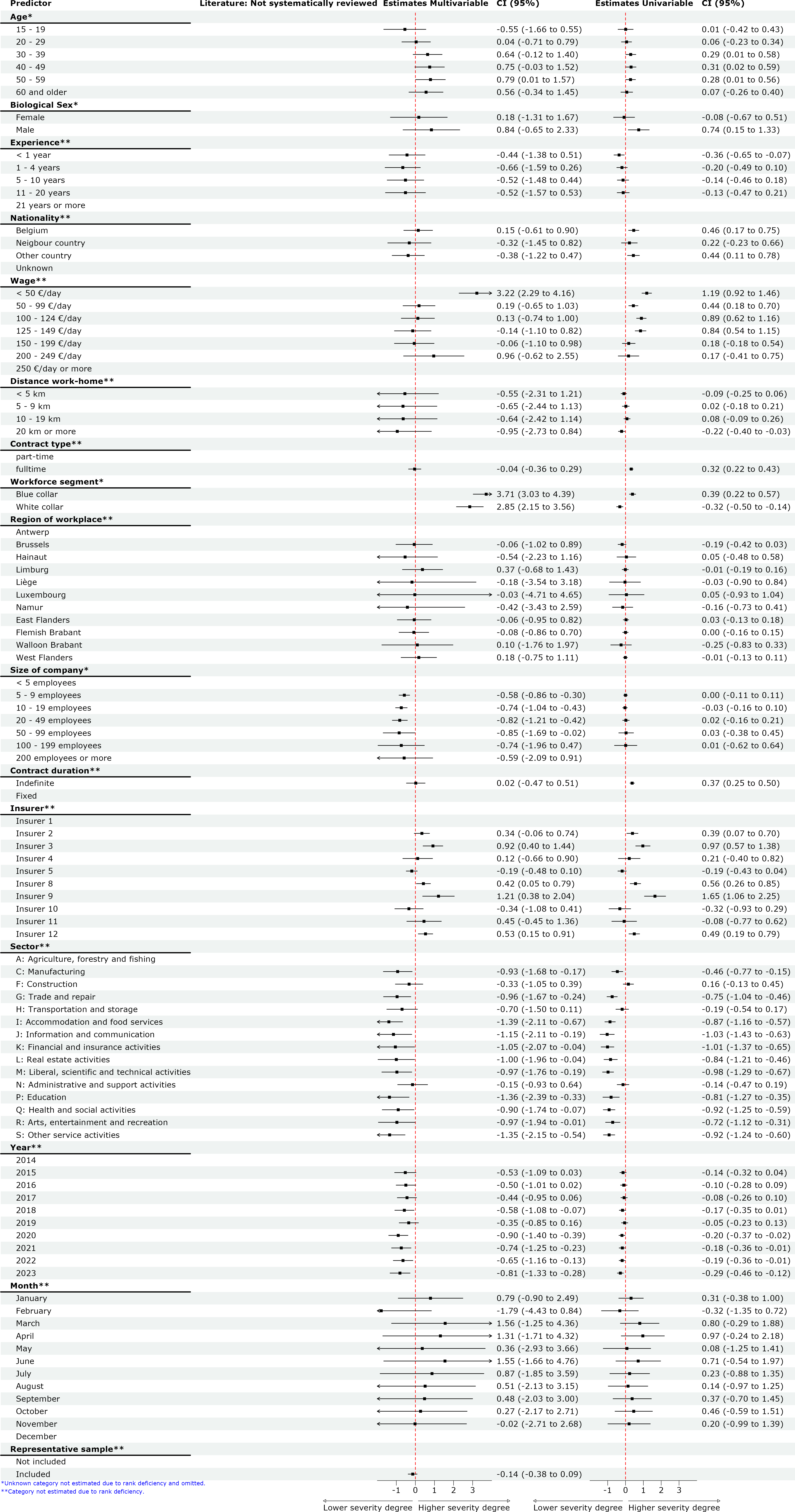
3.5.14 Summary overview of the discussed multivariable models
A summary overview of all multivariable models can be found in Table 3.146. In this table, the model quality of the of all discussed models is compared. For model 2 (Section 3.5.3), conditional R², R² ratio and ICC are presented between parentheses since they were estimated using data from the null model (see Figure 3.224).
Models 1 (Section 3.5.1), 1.1 (Section 3.5.2), 2 (Section 3.5.3), 3 (Section 3.5.4), and 5 (Section 3.5.7) are logistic regression models. A major distinction between these and many studies discussed in the literature review and earlier sections is the scope of the population analysed. In Models 1, 2, and 3 of the present study, we aimed to include all workers occupationally exposed to the risk of experiencing an OA, whereas many other studies focus solely on workers who have already experienced such accidents. This difference in population scope can distort our understanding of the relative importance of various determinants, as the distribution of characteristics in the general working population may differ substantially from that of the subpopulation affected by OAs.
Among Models 1, 2, and 3, Models 1 and 3 show relatively high marginal R² and R² ratios. This similarity is expected, given that approximately 85% of all OA are workplace-related. The high marginal R² values (in bold) suggest that these models explain a larger portion of the variance in the outcome variable, making them more informative and useful for understanding accident occurrence.
In contrast, the performance gap between Model 3 and Models 4 and 8 is substantial, particularly in terms of marginal R². Model 4, which examines the frequency degree of workplace OA at the company level per year, has a much lower marginal R², indicating limited explanatory power. The discrepancy is even more pronounced when considering conditional R² and the ICC: over 90% of the variance in frequency degrees remains unexplained by Model 4 and appears to lie within companies over time rather than between companies. This suggests that while workplace OA occurrence can be reasonably explained using individual- and company-level determinants (as in Model 3) on a monthly basis, this is not the case for company-level frequency degree patterns gathered at year basis.
Models 6 and 6.1 aim to explain variance in the duration of temporary absence following an occupational accident (OA), but differ in how the outcome variable is constructed. Model 6 (nDaysTAO) relies on absence data provided by the insurer, whereas Model 6.1 (lengtecor) calculates absence duration based on payroll records, which may offer a more accurate representation of actual absence. The marginal R² values (Model 6: 0.200; Model 6.1: 0.111) suggest that the fixed effects in Model 6 account for a larger portion of the variance in absence duration than those in Model 6.1. In contrast, the conditional R² values (Model 6: 0.330; Model 6.1: 0.381) indicate that Model 6.1 performs slightly better when random effects, such as company-level variation, are taken into account. This suggests that the payroll-based measure may be more sensitive to organizational context, potentially reflecting differences in how absence is recorded, managed, or influenced by internal company practices. The higher marginal R² in Model 6 likely reflects the standardized nature of insurer reporting, which aligns well with the fixed effects used. Meanwhile, the higher conditional R² in Model 6.1 implies that payroll-derived absence data may better capture contextual or structural influences, even if it is less predictable from fixed effects alone.
Model 7 aims to explain variance in the cost of occupational accidents (OA), using a transformed continuous outcome variable (\(\log_{10}(\text{costOA} + \text{€}1)\)). This transformation helps normalize the distribution of cost data. The model shows a marginal R² of 0.153, indicating that the fixed effects explain a moderate portion of the variance in OA-related costs. The conditional R² is higher at 0.378, suggesting that company-level random effects contribute meaningfully to the overall explanatory power. This pattern implies that while individual and accident-level predictors offer some insight into cost variation, a substantial part of the variance is structured at the organizational level. The ICC of 0.27 further supports this, pointing to clustering of cost outcomes within companies. These results highlight the importance of organizational context in shaping the financial impact of occupational accidents, and suggest that uncaptured company-specific factors (e.g. safety culture, wage policies,…), may play a significant role in cost outcomes.
Similar conclusions as for Model 4 apply to Model 8, which attempts to explain variance in yearly company severity degrees. These findings call for caution when using frequency or severity degree metrics to guide management decisions, shape company safety policies, or inform governmental and insurance frameworks for setting fees or fines. Like already clarified in the previous discussion section, overreliance on these measures may lead to misguided interventions if the underlying variability is not adequately captured.
| Parameter | mod1 | mod1.1 | mod2 | mod3 | mod4 | mod5 | mod6 | mod6.1 | mod7 | mod8 | mod8.1 |
|---|---|---|---|---|---|---|---|---|---|---|---|
| outcome | hadOA | statusOA | comOA | wplOA | freqOA | seriousOA | nDaysTAO | lengtecor | costOA | sevOAval | sevOAcal |
| type | odds ratios | odds ratios | odds ratios | odds ratios | est. | odds ratios | incid. rate ratios | incid. rate ratios | est. (log10+1) | est. | est. |
| R² marg. | 0.136 | 0.001 | 0.183 | 0.146 | 0.058 | 0.005 | 0.200 | 0.111 | 0.153 | 0.010 | 0.007 |
| R² cond. | 0.328 | 0.990 | (0.951) | 0.361 | 0.092 | 0.994 | 0.330 | 0.381 | 0.378 | 0.016 | 0.016 |
| R² ratio | 0.41 | 0.00 | (0.19) | 0.40 | 0.63 | 0.01 | 0.61 | 0.29 | 0.40 | 0.63 | 0.44 |
| sigma2 | 3.29 | 3.29 | 3.29 | 3.29 | 2910.01 | 3.29 | 1.52 | 0.95 | 1.30 | 147.42 | 169.16 |
| tau00 crbnr | 0.19 | 0.00 | 0.00 | 0.20 | 111.38 | 4.14 | 0.30 | 0.41 | 0.47 | 0.88 | 1.51 |
| tau00 insznr | 0.76 | 329.80 | 52.45 | 0.91 | 552.81 | ||||||
| ICC | 0.22 | 0.99 | (0.95) | 0.25 | 0.04 | 0.99 | 0.16 | 0.30 | 0.27 | 0.01 | 0.01 |
| N obs | 7938537 | 31645 | 7938537 | 7938537 | 81780 | 17267 | 17287 | 9822 | 20423 | 82989 | 83000 |
| N crbnr | 16362 | 7218 | 16362 | 16362 | 17670 | 4154 | 4168 | 2946 | 4105 | 17735 | 17740 |
| N insznr | 291661 | 25200 | 291661 | 291661 | 14198 | ||||||
| 0 | 7906715 | 28848 | 7934355 | 7913871 | 16131 | ||||||
| 1 | 31822 | 2797 | 4182 | 24666 | 1136 | ||||||
| rate | 0.004 | 0.088 | 0.001 | 0.003 | 0.066 |
Insights from the multivariable models overview
- Broader population scope for likelihood modelling is an added value. Models 1, 2, and 3 include all workers exposed to OA risk, unlike many studies that focus only on those already affected. These likelihood models yield a more realistic view of the full range of determinants.
- Strong explanatory power for individual-level OA occurrence models. Models 1 and 3 show high marginal R² and R² ratios, indicating they effectively explain notifications (Model 1) and workplace-related accepted OA (Model 3). Their similar performance is unsurprising, given that 85% of accepted OA are workplace-related.
- Limited insights from company-year level models call for caution regarding frequency and severity degrees. Model 4 (OA frequency degree per company per year) and Models 8/8.1 (OA severity degree per company per year) show low marginal and conditional R², suggesting most variance lies within companies over time, not between them. The poor explanatory power indicates these metrics may be unreliable for policy or management decisions.
- Data source impacts model performance for absence duration modelling. Model 6 (FEDRIS-validated data) explains more variance via fixed effects, while Model 6.1 (payroll data) captures more company-level variation. Differences in model quality show how data origin affects explanatory power and sensitivity to organizational context.
- Cost of OA is company-dependent. Model 7 shows moderate fixed-effect explanatory power but strong company-level clustering, implying that organizational factors heavily influence OA-related costs.
- Low explanatory power models still yield important information. Models assessing whether an accepted workplace OA is classified as serious (Model 5) or whether a notified OA is refused (Model 1.1) show very high conditional R² but extremely low marginal R². This indicates strong clustering effects (e.g., company-level variation) but weak predictability from the fixed effects included in the models. Importantly, this does not imply flawed analysis. The study deliberately focuses on the role of determinants (antecedents), excluding OA-specific circumstances. These models still offer meaningful conclusions: the included determinants appear to play little to no role in influencing refusal or seriousness classification decisions. In other words, they are not sources of discrimination, a valuable finding in itself.
- Random effects matter. Several models (e.g., 6/6.1, 7) show that company-level random effects significantly contribute to outcome variance, underscoring the importance of organizational context. Mixed-effects modelling is not just a tool for statisticians, it is a crucial approach for capturing real-world complexities in OA analyses.
3.6 Strengths and limitations of the study
A broad and large study. The present study is broad and large. We investigated a large number of OA (>200k), across multiple NACE-BEL-2008 sectors (>20), happening in many companies (48k – 69k), in a large population of exposed workers (>600k), in a substantial timespan (ten years). In this ways, the study is able to fill significant gaps (see Section 1.4).
Mixed model approach. The application of a mixed-effects model approach to predict the individual likelihoods of reporting an OA or having a commuting or workplace OA represents a significant methodological advancement over existing research, which predominantly relies on aggregated descriptive statistics of OA that already took place. By accounting for repeated observations within individuals and clustering within companies, this approach corrects for the non-independence of observations, thereby reducing bias in parameter estimates and standard errors. Furthermore, our models enable the decomposition of variance across multiple hierarchical levels, offering insights into whether reporting an OA is primarily driven by individual characteristics or organizational factors. This multilevel perspective not only enhances explanatory power but also provides actionable intelligence for targeted prevention strategies, a dimension largely absent from current national reporting systems.
Correction for a representative sample. An extra variable was included in all models to correct for the non-representative distribution of Liantis mutual ESPP and PS customers across Belgian provinces, sectors and company size. This correction enhances the generalizability of our findings to the broader Belgian working population, addressing a common limitation in OA research where samples may not accurately reflect the diversity of the workforce.
Including insurers as a determinant. To our knowledge, this is the first study in which the OA insurer is included as a determinant for a broad series of relevant outcomes. In this way, our study is highly relevant in filling a significant gap in the literature.
External benchmarking. By comparing our study sample with official statistics from NSSO and FEDRIS, we were able to benchmark our findings against established national data sources. This external validation strengthens the credibility of our results and places them within the broader context of OA research in Belgium. However, this approach also introduces a limitation. To align with the categorisations used in these official datasets, we had to simplify or recode certain variables, resulting in a loss of granularity. Variables such as age, wage, and company size, for instance, could have been treated as continuous variables as well, potentially leading to more nuanced and statistically powerful models.
No analysis at the accident mechanism level. This study does not include an analysis of specific accident mechanisms (e.g., falls from height, machinery-related incidents). Although such details are recorded once an OA has occurred, we deliberately chose to exclude them from our analyses. The primary reason is that this information is only available for individuals who have already experienced an OA. Including these variables would restrict the analysis to a subset of the workforce, potentially introducing selection bias and limiting the generalizability of our findings. Our focus was on identifying determinants of OA occurrence and outcomes across the entire exposed workforce, rather than examining the specific circumstances of accidents post-occurrence. While future research could explore accident mechanisms in greater detail, this study prioritizes a broader perspective on OA.
Waterfall loss. For likelihood modelling, information was also needed from employees not experiencing any OA. The availability of this necessary detailed information reduced the potential of 69,157 Liantis ESPP only employers to 47,820 Liantis ESPP and PS mutual customers. As a consequence, the original 293,938 ESPP only notifications were reduced to 90,619 notifications from 52,240 unique employees within mutual Liantis ESPP and PS customers. From this point on, further reduction to achieve complete cases for all determinants included in the models could be necessary (e.g. mod1.1 25,200 unique individuals left).
Underreporting bias. A recent systematic review investigated underreporting of OA (Kyung et al., 2023). While across the world several government based (regulatory compliance) and insurer/compensation based (financial benefits) reporting systems co-exist, underreporting risks are overall very high. Multiple studies across diverse industries and countries found rates ranging from 20% to over 90%, depending on the sector, injury severity, and reporting system. Belgium relies in first instance on a compensation based system. In such a system, underreporting occurs when workers fear retaliation, lack awareness, or perceive the claims process as burdensome. Some studies show that not all workplace injuries are reported to insurers, especially less severe cases, due to these barriers (Azaroff et al., 2002). Figure 2.1 reminds us of this the tip of the iceberg problem: incidents and light accidents are de facto not included in the study. For all other accidents, the choices of multiple actors during the notification process can influence whether the OA will actually be notified or not. It is crucial to keep this underreporting bias throughout the whole study in mind when interpreting the results. However, since the underreporting problem of OA is present in many published studies, we expect our results to be comparable and complementary to existing scientific literature.
Including insurers as a determinant. Insurers associated with companies that did not report OA may be underrepresented in the dataset, as insurer information is only reliably available for cases where the company was a client of Liantis Risk Solutions. In other cases, the insurer was inferred retrospectively via the FEDRIS Fonds voor Arbeidsongevallen (old Dutch name of FEDRIS before the fusion with FBZ, FAT in French) (FAO) number following the occurrence and notification of an OA. And although including the insurer as a determinant can be regarded as a strength of our study leading to new insights, it can also introduce bias and certainly reduced the number of due to the necessity of complete cases for modelling.
Excluding certain sectors. Although we aimed to include all NACE-BEL-2008 sectors, some sectors had to be excluded due to insufficient data availability. For example, the public sector is largely absent from the dataset since Liantis primarily serves private sector employers. Also mixed private/public sectors proved to be difficult to include. Our study thus does not provide insights in the level 1 sectors B, D, E, O, U and T.
Collapsed categories. Unlike the NSSO and FEDRIS statistics, which cover the entire Belgian population, this study is limited to the mutual clients of Liantis ESPP and PS. As with sector classifications, certain categories of key variables used in official statistics may be underrepresented or overrepresented in this dataset. When these variables are cross-tabulated with other important determinants, small or empty cells can occur, which may prevent statistical models from converging. A clear example is company size: while the univariable analysis (see Section 3.4.3.2) allowed for detailed categories such as 200–499, 500–999, and 1000+ employees, the multivariable models (see Section 3.5) failed to converge with this level of granularity. As a result, all categories with 200 or more employees had to be collapsed into a single group.
Wage category interpretation. One important limitation in this study concerns the interpretation of wage categories, particularly the lowest category (e.g., less than €50/day). This group differs significantly from the other wage categories and should be interpreted with caution. Due to the nature of the available raw payroll data, it was not possible for every record to verify to what extent the reported wage figures reflect actual gross salary levels. Wage calculations are inherently complex and influenced by a variety of contextual factors. For instance, low reported wages may not necessarily reflect low compensation, but rather periods of long-term absence, such as extended sick leave or disability. In such cases, the employee remains formally employed but is not actively working, and therefore not exposed to occupational risks. Additionally, during these absence periods, wage costs may no longer be borne directly by the employer, as compensation may be covered by social security mechanisms. Furthermore, a significant data quality issue must be acknowledged regarding the lowest wage category. A gross wage of less than €50 per day is not realistic in today’s context and likely results from anomalies in the dataset. These anomalies include records with extremely low or zero wages, which may be linked to specific employment statutes that could not be traced during the analysis. Examples include certain learning contracts or company directors/entrepreneurs with reported wages of €0. While such cases were present in the database, they could not be reliably identified or excluded. Therefore, this lowest category should not be considered a true representation of low-wage workers, but rather a heterogeneous group with mixed characteristics. Another layer of complexity arises from the temporal scope of the dataset, which spans multiple years. Wages from 2014 are not directly comparable to those from 2023, as indexation and inflation are not taken into account. This limits the interpretability of absolute wage values over time. Therefore, it is essential to focus on the relative positioning of wage categories within the model, rather than on their absolute numeric values or coefficients. Interpreting wage categories in relative terms provides a more robust and meaningful understanding of their role in the analysis.
Excluding OA specific variables without counterpart. A final limitation of this study is the exclusion of certain informative, accident-specific variables from the multivariable models. Factors such as shift work, long working hours, usual professional activity, specific task at the time of the accident, and type of workstation are known to significantly influence occupational accident outcomes. However, these variables could not be included due to the lack of structurally available counterparts for workers in the Liantis mutual ESPP and PS customer base who did not experience an OA. Without comparable data for the non-accident group, including these variables would have introduced bias and undermined the validity of the models.
List Of Acronyms
- CBE
- Crossroads Bank for Enterprises (KBO in Dutch)
- COVID-19
- Coronavirus Disease 2019
- ESAW
- European Statistics on Accidents at Work
- ESPP
- External Service for Prevention and Protection at work (EDPB in Dutch)
- FAO
- Fonds voor Arbeidsongevallen (old Dutch name of FEDRIS before the fusion with FBZ, FAT in French)
- FEDRIS
- Federaal agentschap voor beroepsrisico’s
- GMQ
- General Medical Questionnaire (AMV in Dutch)
- ICC
- Intraclass Correlation Coefficient
- INSZ
- Identificatienummer Sociale Zekerheid (rijksregisternummer of BIS-registernummer)
- IRR
- Incidence Rate Ratio
- ISCO
- International Standard Classification of Occupations
- NACE-BEL
- Belgian version of the the Europese activiteitennomenclatuur (NACE)
- NIS
- Nationaal Instituut voor de Statistiek
- NSSO
- National Social Security Office
- OA
- Occupational Accident
- OR
- Odds Ratio
- PC
- Paritair Comité (joint collective agreement or sectoral committee)
- PPE
- Personal Protective Equipment
- PS
- Payroll Services
- RS
- Risk Solutions
- RSZ
- Rijksdienst voor Sociale Zekerheid
- SEATS
- Signal Extraction in Arima Time Series
- TRIR
- Total Recordable Incident Rate
- crbnr
- enterprise identification number within CBE
- insznr
- personal identification number within NSSO (INSZ number)